May 26, 2016 - Yun-Chung Chung (é¾å
ä¸) received the B.E. degree in Naval ... degree in Biomedical Science from Oakland University, Rochester, ... Ford Hospital, Detroit, Michigan, USA, and working in the area of medical physics. Then ...
JOURNAL OF INFORMATION SCIENCE AND ENGINEERING 25, 1939-1953 (2009)
Short Paper__________________________________________________ Intrinsic Image Extraction from a Single Image YUN-CHUNG CHUNG, SHEN CHERNG*, ROBERT R. BAILEY AND SEI-WANG CHEN Department of Computer Science and Information Engineering National Taiwan Normal University Taipei, 116 Taiwan * Department of Computer Science and Information Engineering Cheng Shin University Kaohsiung, 833 Taiwan An image is often modeled as a product of two principal components: illumination and reflectance components. The former is related to the amount of light incident on the scene and the latter is associated with the scene characteristics. The images formed from the two components are referred to as the illumination and the reflectance images; both are called the intrinsic images of the original image. The illumination components of the images of a fixed scene vary from image to image, while the reflectance components of the images in principle remain constant. Both reflectance and illumination images have their own applications. Intrinsic image extraction has long been an important task for computer vision applications. However, this task is not at all simple because it is an illconditioned problem. The proposed approach convolves an input image with a prescribed set of derivative filters. The pixels of the derivative images are next classified as being reflectance or illumination according to three measures: chromatic, intensity contrast and edge sharpness, which are calculated in advance for each pixel from the input image. Finally, a de-convolution process is applied to the classified derivative images to obtain the intrinsic images. The results reveal the feasibility of the proposed technique in both rapidly and effectively decomposing intrinsic images from one single image. Keywords: reflectance and illumination components, intrinsic images, intensity contrast and edge sharpness measures, photometric reflectance model, chromatic measurement
1. INTRODUCTION The intensity of an image reveals the brightness of a scene, which in turn is determined by two major factors, one associated with the amount of light incident on the scene and the other related to the reflectance of the scene. As a consequence, an image is often modeled as a product of two comp onents: illumination and reflectance components [10, 25, 29], which correspond to the two factors, respectively. The images formed from these two components are referred to as the illumination image and the reflectance image, and are jointly called the intrinsic images [2, 12, 19, 24] of the original image. In many computer vision applications, it is desirable that the reflectance and illumination components be decomposed from the input image. Both components have their own advantages. Since the reflectance component is related to the scene characteristic, Received December 24, 2007; revised June 27, 2008; accepted August 22, 2008. Communicated by Tong-Yee Lee.
1939
1940
YUN-CHUNG CHUNG, SHEN CHERNG, ROBERT R. BAILEY AND SEI-WANG CHEN
the reflectance image in principle remains constant under different illumination conditions. For applications such as object recognition [4], pattern classification [18], scene interpretation [8], and visual surveillance [20, 27], it is preferable to use reflectance images. The illumination component varying with different lighting conditions can be used for tasks such as illumination assessment [7, 13], shading analysis [3, 14, 21], color constancy [11], and geometric modeling [22]. Decomposing an image into its reflectance and illumination components is an ill-posed problem [2]. There are two unknowns (illumination and reflectance components) that are to be derived from one given data (the input image). Additional information is needed to separate the components. Weiss [28] used multiple images. Let Ii (i = 1, …, n) be a set of images taken of a scene under different illumination conditions. Since the reflectance component is assumed to be constant, say R, a set of n equations, Ii = R × Li (i = 1, …, n), can be constructed, where Li is the illumination component of image Ii. However, this set of n equations is still not enough to solve for the n + 1 unknowns (R and Li). Weiss further introduced a sparseness assumption [23], which states that the filtered images obtained by applying gradient operators to the input images are sparse (i.e., they contain mostly zeros) so that the histograms of the filtered images can be fitted with a Laplacian function. With this assumption, the decomposition problem becomes solvable. Weiss then estimated R and Li using a maximum likelihood technique. Yuille et al. [29] also used as the input data a set of images taken of an object under different and unknown lighting conditions. A singular value decomposition technique was applied to the images to separate the images into components depending on surface characteristics (geometry and albedo) and illumination conditions. Based on the extracted surface characteristics, a generative model of the object [15], which approximates the object’s appearance under a restricted range of illumination conditions, was determined. Since multiple images were used, the applicability of their techniques is somewhat limited. Tappen et al. [26] proposed a method for recovering intrinsic components from a single image. A set of derivative filters are first applied to the input image giving rise to a set of derivative images. The pixels of the derivative images are classified as being reflectance or illumination based on their color and intensity. However, unsatisfactory results were observed. Tappen introduced a process, called the generalized belief propagation process, to improve the results. Next, a de-convolution process was applied to the classified derivative images to obtain the intrinsic images of the input image. The Tappen method took about six minutes to categorize pixels and another six minutes to perform the generalized belief propagation process. To use with real-time applications, the time complexity of the Tappen method should be significantly reduced. Recently, Matsushita et al. [20] introduced an illumination eigenspace into Tappen’s computational framework. The eigenspace, which is built in advance, provides information for categorizing the pixels of derivative images. Since no information is computed during pixel classification, the Matsushita approach can operate in real time. However, over a period of 120 days Matsushita collected a set of 2048 images from a scene for generating its illumination eigenspace. Apparently, Matsushita’s method can not be applied to time-varying scenes (i.e., dynamic scenes). To be applicable to dynamic scenes, the information for classifying pixels of derivative images must be computed directly from the input image, and for real-time applications, the computation should be efficient. In [17], the normalized RGB color space is used as the chromaticity to produce
INTRINSIC IMAGE EXTRACTION FROM A SINGLE IMAGE
1941
weighted edge maps to classify the edges of the input image. However; the evidence from such simple chromaticity is not reliable in many conditions. In addition, an illuminationinvariant image is used to recover intrinsic images in [9]. Both information selection and classification strategy play critical roles in determining the goodness of classification results, which in turn determines the robustness of the proposed intrinsic image decomposition method. In this study, three measures (chromatic, intensity contrast and edge sharpness) and a hierarchical classification strategy are proposed for classifying the pixels of derivative images. The details of the overall process of intrinsic image decomposition are given in section 2. Section 3 is devoted to a discussion of invariant chromatic characteristics that are used to define the chromatic measure. Experimental results are presented in section 4 and concluding remarks and future work in sections 5.
Fig. 1. Proposed flowchart for extracting intrinsic images from a single image.
2. INTRINSIC IMAGE DECOMPOSITION Fig. 1 shows a flowchart for the proposed approach to extracting intrinsic images from a single color image. The approach consists of four major stages: logarithmic edge generation, characteristic measure calculation, edge classification, and intrinsic image formation. Let I = (Ir, Ig, Ib) denote the input color image, where Ir, Ig and Ib are the red, green and blue components of the input image. Each color component Ii is modeled as Ii = Ri × Li, where Ri (reflectance) and Li (illumination) are the intrinsic images of Ii. The process of Fig. 1 is applied to each of the color components. The intrinsic images, R and
1942
YUN-CHUNG CHUNG, SHEN CHERNG, ROBERT R. BAILEY AND SEI-WANG CHEN
L, of the input image are finally formed from Ri and Li by R = (Rr, Rg, Rb), L = (Lr, Lg, Lb). 2.1 Logarithmic Edge Generation Let Ii be any color component image. In the logarithmic edge generation stage, Ii is first transformed into the logarithmic domain, Ii′ = logIi = log(Ri × Li) = logRi + logLi = Ri′ + Li′,
(1)
resulting in an additive composition of reflectance and illumination. This also reduces the dynamic range of Ii so as to increase its intensity contrast. The transformed image Ii′ is next convolved with a horizontal derivative filter fh and a vertical derivative filter fv, rei i sulting in two derivative component images I h′ and I v′. In this study, the Prewitt derivative filters are utilized. From the derivative component images, an edge map Ei of size r × c is generated, which is the same as the image size. Each element e of map Ei contains a derivative magnitude mi(e) and a derivative orientation oi(e), where
mi (e) = ( I hi ′2 (e) + I vi ′2 (e))1/2 and oi (e) = tan −1 ( I hi ′ (e) + I vi ′ (e)).
(2)
2.2 Characteristic Measure Calculation
In the second stage of characteristic measure calculation, three measures, chromatic, intensity contrast and edge sharpness, are calculated for each image pixel. The calculated measures will be used in the next stage for classifying the pixels of derivative component images into illumination or reflectance edge pixels. In the following, pixels are temporarily treated as edge pixels when calculating their characteristic measures. 2.2.1 Chromatic measure, A
Consider a pixel p and let wp be a neighborhood window centered at p. We look for a straight line l passing through p within wp. The line is formed from the pixels whose sum of derivative magnitudes is maximal. This line divides wp into two regions, say w1 and w2. To calculate the chromatic measure of p, for each pair of pixels (pi, pj) in w1 and w2, the correlation cij of the chromatic characteristic (given in section 3) between the two pixels pi and pj is calculated. Let Ci and Cj be the vectors formed from the chromatic characteristics of pixels pi and pj, respectively. The chromatic correlation cij between pi and pj is calculated by cij = Ci ⋅ Cj/(||Ci||||Cj||). Let {cij} be the set of chromatic correlations of all pairs of pixels from the regions w1 and w2. The chromatic measure of pixel p is defined as the median of {cij}. The resulting array of characteristic measure is called the chromatic measure map, and denoted by Ai. 2.2.2 Intensity contrast measure, T
The intensity averages, a1 and a2, of the pixels in regions w1 and w2 are computed. The intensity contrast measure of p is defined as |a1 − a2|/kI, where kI normalizes |a1 − a2| so that the intensity contrast measures are between 0 and 1. The intensity contrast measure map of the entire image is denoted by TiI.
INTRINSIC IMAGE EXTRACTION FROM A SINGLE IMAGE
1943
2.2.3 Edge sharpness measure, S
First, we find the line l′ perpendicular to the previously found line l. Next, along l′ we compute the standard deviation σi of derivative magnitudes of pixels within wp, σi(p) = ( 1n ∑ |mi ( p ′) − mi |2 )1/2 , where n is the number of pixels and mi is the mean of their p′
derivative magnitudes. The edge sharpness measure of pixel p is defined as the normalized product of its derivative magnitude mi and its standard deviation σ i of the derivative magnitudes, mi(p)σi(p)/kS, where kS normalizes the values to between 0 and 1. Clearly, the larger both mi(p) and σi(p) are for an edge pixel, the sharper the edge pixel will be. Let Si be the edge sharpness measure map, which contains the edge sharpness measures of all pixels. More details can be found in [6]. 2.3 Hierarchical Edge Classification
In the edge classification stage, the measures calculated in the previous stages are i i used to classify the pixels of derivative component images I h′ and I v′ as reflectance or illumination edge pixels. Fig. 2 shows the classification process for some pixel p. First, we inspect its derivative magnitude mi(p). If mi(p) exceeds a threshold tm, p is a potential edge pixel. We then examine its intensity contrast measure T i(p). A small T i(p) indicates a small difference in intensity between the two sides of p, in which case we classify p as a reflectance edge pixel. Refer to Fig. 3, where a polyhedron sitting on a horizontal surface is illuminated by a distant light source located to the upper left of the polyhedron. A line FG, which is drawn on a face of the polyhedron, does not result from an illumination gradient; it has a small intensity contrast measure and, hence, is a reflectance edge. Similarly, polyhedral edges AI, BC and HC, which are reflectance edges, all have small intensity contrast measures. On the other hand, if pixel p has a large intensity contrast measure, the pixel may be an illumination or a reflectance edge pixel. Edges AB and BE in Fig. 3 both have large intensity contrast measures. However, AB is a reflectance edge because it is an object edge, while BE is an illumination edge because it is created by a difference of illumination between its two sides. To determine the edge type of pixel p, we need an additional measure. Consider the chromatic measure Ai(p) of p. If Ai(p) is small, i.e., the difference between the chromatic characteristic of the two sides is large, pixel p is classified as a reflectance edge pixel. See edge DH in Fig. 3, which is a reflectance edge because it separates the polyhedron from the background. Most often, different objects have distinct surface characteristics and the correlation of their surface characteristics will be small. However, it is possible that two objects happen to have similar surface characteristics. In this case, we appeal to the sharpness measure of the edge separating the two objects. If the edge sharpness measure is large, we classify the edge as reflectance and otherwise as illumination. Edges AB (a reflectance edge) and BE (an illumination edge) in Fig. 3 both have large intensity contrast measures and large chromatic measures. Based on these two measures, we will not be able to determine their edge types. But, if its edge sharpness measure is large, we will classify an edge as reflectance, and otherwise as illumination. The above edge classification process can successfully interpret the edge types of all the line segments in Fig. 3. However, in reality various complicated situations may
1944
YUN-CHUNG CHUNG, SHEN CHERNG, ROBERT R. BAILEY AND SEI-WANG CHEN
Fig. 2. Hierarchical edge classification process.
Fig. 3. Example for illustrating edge classification.
occur, such as specularities, inter-reflections, and scenes that are too bright or too dark. These can result in indeterminate or numerically unreliable values for characteristic measures. Therefore, we restrict ourselves to outdoor scenes during daytime and scenes without very high or very low brightness. Note that outdoor scenes provide ample fields of view for cameras so that the portion of specularities is very small relative to the entire scene. During the classification process, some pixels have not been classified. For these pixels, we introduce an evidence following process which incrementally determines their edge types through progressive propagations of local evidence. Let Gi be the array, called the classification map, which contains the classification results of all pixels. Let e be some element of the map whose edge type has not yet been determined. Examining edge map Ei, let mi(e) and oi(e) be the derivative magnitude and derivative orientation of e. We check its two adjacent neighbors, say n1 and n2, in the direction oi(e) and select the one
INTRINSIC IMAGE EXTRACTION FROM A SINGLE IMAGE
1945
with the larger derivative magnitude. If the edge type of the selected neighbor has been decided, we set Gi(e) to the edge type of that neighbor,
G i (e) = arg (max{mi (n1 ), mi (n2 )}).
(3)
G i ( ni )
However, if the neighbor has not yet been classified, we continue to the next undetermined element of Gi. The above process is repeated until all elements of Gi are classified. This completes the evidence following. After this, every element of Gi contains a symbol, either sR or sI, which denote reflectance- and illumination edge types, respectively. The classification maps, Gi (i = r, g, b), obtained from different color components may not be mutually consistent. We say a pixel is ambiguous if it has different edge types in the three classification maps. For such a pixel, we use a vote to decide a unique edge type for the pixel. Let p be such an ambiguous pixel. We add up its derivative magnitudes to obtain sums SR(p) and SI(p) according to the edge types of the pixel determined in the classification maps, i.e., S R ( p ) = ∑ ∑ mi ( p) and S I ( p) = ∑ ∑ mi ( p). i = r , g ,b G i ( p ) = S R
i = r , g ,b G i ( p ) = S I
We then decide the edge type of p in map G by G ( p ) = arg (max{S R ( p ), S I ( p )}). For SR , SI
non-ambiguous pixels, we simply copy their edge types to map G. i i Based on the resultant classification map MG, we generate reflectance R h, R v and i i i illumination Lh, Lv derivative component images from derivative component images I h′ i′ and I v . For a pixel p, if G(p) = sR, then Rhi ( p ) = I hi ' ( p ), Rvi ( p ) = I vi ' ( p ) and Lih ( p ) = 0, Liv ( p ) = 0; if G(p) = sI, then Rhi ( p ) = 0, Rvi ( p ) = 0 and Lih ( p ) = I hi ' ( p ), Liv ( p ) = I vi ' ( p ).
(4)
This step separates derivative component images as reflectance or illumination, and i i i i R h, R v, R h, and Lv are called the intrinsic derivative component images. 2.4 Intrinsic Image Formation
At the final stage of intrinsic image formation, de-convolution [28] is applied to the intrinsic derivative component images, from which the logarithmic reflectance Ri′ and illumination Li′ component images are computed,
Ri′ = g *(
∑
j = h,v
f jr * Rij ), Li′ = g * (
∑
j = h ,v
f jr * Lij ),
(5)
where fjr is the reversed function of fj defined as fjr(p) = fj(− p). The symbol * denotes discrete convolution, and g is a normalization term satisfying
g ∗(
∑
j = h,v
f jr ∗ f j ) = δ ,
(6)
where δ is the Kronecker delta function. To compute Ri′, we convolve both sides of Eq. (5) with ∑ f jr ∗ f j , and get j = h,v
YUN-CHUNG CHUNG, SHEN CHERNG, ROBERT R. BAILEY AND SEI-WANG CHEN
1946
(
∑
j = h,v
f jr ∗ f j ) ∗ R i′ =
∑
j = h,v
f jr * R ij .
Applying the Fourier transform ℑ to the above equation, ℑ((
∑
j = h,v
f jr ∗ f j ) ∗ R i′ ) = ℑ(
∑
j = h ,v
f jr * R ij ).
(7)
By the convolution theorem, Ri′ = ℑ−1 (ℑ( ∑ f jr * R ij ) / ℑ( ∑ f jr ∗ f j )), where ℑ-1 is the j = h ,v j = h,v inverse Fourier transform. Likewise,
Li′ = ℑ−1 (ℑ(
∑
j = h,v
f jr * Lij ) / ℑ(
∑
j = h ,v
f jr ∗ f j )).
(8)
Finally, we apply the exponential transform to the logarithmic intrinsic component images Ri′ and Li′. The reflectance Ri and illumination Li component images of the color component image Ii are obtained by Ri = exp(Ri′) and Li = exp(Li′). After obtaining the intrinsic component images of the (r, g, b) three color component images, Ri and Li, the intrinsic images, R and L, are formed from R = (Rr, Rg, Rb), L = (Lr, Lg, Lb).
3. CHROMATIC CHARACTERISTICS For calculating chromatic measures of image pixels, we need to know the chromatic characteristics of pixels in advance. Many chromatic characteristics that are invariant to scene geometry and incident illumination have been proposed in the literature [1, 16]. In this study, four groups of chromatic characteristics, denoted by H, C, W and N, which can be efficiently calculated from the input image, are considered. Rather than using all the invariant chromatic characteristics suggested by Geusebroek [16], eleven chromatic characteristics, H, Hp, C, Cλ, Cp, Cλp, W, Wλ, Wλλ, N, and Nλ, are adopted for this study. They are given below and in Eq. (9),
H p = H v2 + H h2 , where H i =
Eλλ Eλ − Eλ Eλλ i , i = v, h, 2 Eλ2 + Eλλ
Eλλ E E−E E , C p = Cv2 + Ch2 , where Ci = λ i 2 λ i , E E − E E E E i i λλ λλ , Cλ p = Cλ2v + Cλ2h , where Cλ i = E2 E Wλ = Wλ2v + Wλ2h , where Wλ i = λ i , E Eλλ i 2 + W 2 , where W , Wλλ = Wλλ λλ i = v λλ h E E E 2 − Eλλ Ei E − 2 Eλ i Eλ E + 2 Eλ2 Ei . N λ = N v2 + N h2 , where Ni = λλ i E3 Cλ =
(9)
Each characteristic can be invariant only under certain imaging conditions. Five imaging conditions are considered in this study, uniform illumination, equal energy spec-
INTRINSIC IMAGE EXTRACTION FROM A SINGLE IMAGE
1947
trum, colored illumination, matte, dull surfaces, and uniformly colored surfaces. The first three conditions are related to illumination, and the remaining two are related to object surfaces. Since general scenes are considered in this study, the objects constituting a scene can not be known a priori. The imaging conditions concerning object surfaces become impractical and so do the chromatic characteristics, whose invariance properties are subject to the conditions. In the following, we concentrate on the illumination conditions and the associated chromatic characteristics. Instead of directly considering the three illumination conditions, we turn to three fundamental lighting sources: diffuse, ambient, and direct lightings. Any illumination condition can be approximated as a combination of the three. Diffuse lighting comes from the lights reflected off environmental objects. Ambient lighting results from surrounding light sources. Direct lighting comes from a single intense light source. There are more than 300 color images in the database [33], which were taken of 100 objects under the three lighting conditions. Objects were made of various kinds of materials. We used it to study the properties of chromatic characteristics. Let I1, I2 and I3 be the images of the same scene S taken under diffuse, ambient and direct lighting conditions, respectively. Let C specify any of the above chromatic characteristic and C1(p), C2(p) and C3(p) represent the values of the chromatic characteristic at pixel p for the three images, respectively. Ideally, C1(p) = C2(p) = C3(p), indicating that the chromatic characteristics of the same material are invariant under different lighting conditions. Let σC(p)denote the standard deviation of C1(p), C2(p) and C3(p), i.e.,
σ C ( p) = [
1 3 1 3 (Ci ( p) − C ( p)) 2 ]1/ 2 , where C ( p) = ∑ Ci ( p). ∑ 2 i =1 3 i =1
(10)
We define the degree of invariance of chromatic characteristic C for scene S as AC ( S ) =
np
ε + ∑ σ C ( p)
,
(11)
p
where np is the number of image pixels and ε is a small positive number to prevent the denominator from being zero. From our previous observations result [5], we select chromatic characteristics H, C, Cλ for the experiments of intrinsic image extraction.
4. EXPERIMENTAL RESULTS In the previous section, a number of chromatic characteristics were introduced for calculating chromatic measures of image pixels. The chromatic measure together with the other two measures of intensity contrast and edge sharpness was used to classify the pixels of derivative images into reflectance or illumination edge pixels. The intensity contrast and edge sharpness measures are calculated from intensity values and edge magnitudes, respectively. Compared with chromatic characteristics, intensity values and edge magnitudes are relatively reliable because the calculation of chromatic characteristics involves a number of uncertainties. First, approximate imaging, photometric reflectance, and chromatic measurement models were adopted for calculating chromatic char-
1948
YUN-CHUNG CHUNG, SHEN CHERNG, ROBERT R. BAILEY AND SEI-WANG CHEN
acteristics. Second, high-order spatial and spectral derivatives were involved in the calculation of chromatic characteristics. Third, the invariance properties of chromatic characteristics depend on imaging conditions. Each input image is an RGB color image with a size of 320 by 240 pixels. The output results include a reflectance image and an illumination image extracted from the input image. The source code was written in C++ run on a 2.4 GHz Pentium based PC. The program took about 3 to 4 seconds to decompose an input image into its reflectance and illumination images. Fig. 4 shows three examples of real scenes. The brightness of the reflectance images is lower than that of the input images due to the lack of illumination component in the reflectance images. Also, almost all of the shadows present in the input images were successfully removed from the reflectance images and were assigned to the illumination images. Since shadows often confuse visual systems, reflectance images are useful for applications such as pattern recognition, object classification, scene interpretation, and visual surveillance. On the other hand, illumination images are also useful for such objectives as illumination assessment, shading analysis, color constancy, and object modeling.
(a) Input images. (b) Reflectance images. (c) Illumination images. Fig. 4. Examples using real scenes: column (a) to (c).
Fig. 5 shows more examples of real scenes. Some details, e.g., the characters inscribed on the wall, the left eye of the statue, and the texture on the small ball, all of which are vague due to shadows, become perceptible after removing the shadows (see the reflectance images in the second column of this figure). However, unlike in the reflectance images in Fig. 4 the shadows in Fig. 5 remained shallow yet visible. Although it is possible to eliminate the shadows with the aid of illumination images, we haven’t thus far developed a process that could be general enough to apply to all kinds of images. In the last example in the third row of Fig. 5, there are several blurred areas along the boundaries of the shadow in the illumination image. These areas resulted from errors in the classification of pixels of the derivative image. Recall that our edge classification process categorizes a pixel of a derivative image as being either reflectance or illumination.
INTRINSIC IMAGE EXTRACTION FROM A SINGLE IMAGE
(a) Input images.
1949
(b) Reflectance images. (c) Illumination images. Fig. 5. Examples using real scenes.
However, in reality an edge pixel can be both reflectance and illumination; see for example the input image. The boundaries between long wooden plates are reflectance, while the boundaries created by the shadow are illumination. The pixels located at the intersections between the aforementioned two kinds of boundaries are both reflectance and illumination. Our classification process cannot identify the edge types of those pixels. Moreover, the classification errors are propagated in the course of deconvolution, which causes blurred areas in the illumination image. Fig. 6 shows an example of the importance of edge classification. Fig. 6 (b) presents the result, in which the bright pixels indicate the illumination edge pixels determined by the classification process. There are several broken segments originating from erroneous classifications of the shadow boundary of the person, especially near his legs. The segments result in blurred areas in the illumination image (Fig. 6 (c)). Figs. 6 (d) and (e) show an improved edge classification map using an edge following technique and the associated illumination image, respectively. Several blurred areas in the original illumination image of Fig. 6 (c) were restored in the illumination image of Fig. 6 (e). The above example demonstrates the importance of edge classification. It is also possible to improve the results by applying noise removal to the classification map. Fig. 7 shows the results before and after noise removal. Figs. 7 (b)-(d) shows the edge classification map, the extracted reflectance and illumination images before noise removal, and Figs. 7 (e)-(g) are the results after noise removal. The reflectance image of Fig. 7 (f) contains more reflectance details (both albedo and structure) than that of Fig. 7 (c). However, noise removal may get rid of important clues as well, as can be seen in the illumination image of Fig. 7 (g), in which the shadows of the flowerpot and plants are faded out. In addition, our result is very similar to Fig. 7 (h) [9] but much faster.
1950
YUN-CHUNG CHUNG, SHEN CHERNG, ROBERT R. BAILEY AND SEI-WANG CHEN
(a) Input image.
(a) Input image.
(b) Edge classifi(c) Illumination (d) Improved edge (e) Improved illumication map. image. classification map. nation image. Fig. 6. The importance of edge classification.
(b) Edge classification map. (c) Reflectance image.
(d) Illumination image.
(e) Edge classification map (f) Resulting reflectance (g) Illumination image. (h) Result from [12]. after noise removal. image. Fig. 7. Modify the edge classification result by noise removal.
5. CONCLUDING REMARKS In this paper, an approach to extracting intrinsic images from one single image is presented. Three measures: chromatic, intensity contrast and edge sharpness, which are efficiently calculated from the input image by providing the (R, G, B) values of each pixel, were employed to classify the pixels of derivative images into reflectance or illumination edge pixels. The performance of the proposed approach depends on the goodness of the classification result. In order to improve the classification result, we used a noise removal method and an edge following technique to link broken edges. However, these methods are post-processing. We prefer pre-processing methods, such as increasing the robustness and reliability of the current measures and investigating into new ones. The proposed approach extracts intrinsic images from a single image so that the approach can be applied to images of dynamic scenes. Our method takes about 3 to 4 seconds to complete the intrinsic image decomposition of an image. Compared with the previous methods, the time complexity of the proposed approach has been greatly improved. However, for real-time applications the processing time would be need to further reduced. The edge classification and the intrinsic image formation steps together took about 70% of the entire processing time. Note that there is an evidence following process that is iterative in nature in the edge classification step and that the deconvolution process in the intrinsic image formation step performs an FFT seven times, each taking about 0.1 to
INTRINSIC IMAGE EXTRACTION FROM A SINGLE IMAGE
1951
0.15 seconds. We will concentrate on reducing the processing times of the aforementioned time-consuming processes in our future work.
REFERENCES 1. E. Angelopoulou, S. W. Lee, and R. Bajcsy, “Spectral gradient: A material descriptor invariant to geometry and incident illumination,” in Proceedings of IEEE International Conference on Computer Vision, 1999, pp. 861-867. 2. H. G. Barrow and J. M. Tenenbaum, “Recovering intrinsic scene characteristics from images,” Computer Vision Systems, A. R. Hanson and E. M. Riseman, eds., Academic Press, 1978, pp. 3-26. 3. M. Bell and W. T. Freeman, “Learning local evidence for shading and reflection,” in Proceedings of International Conference on Computer Vision, 2001, pp. 670-677. 4. S. L. Chang, L. S. Chen, Y. C. Chung, and S. W. Chen, “Automatic license plate recognition,” IEEE Transactions on ITS, Vol. 5, 2004, pp. 42-54. 5. Y. C. Chung, S. L. Chang, S. Cherng, and S. W. Chen, “The invariance properties of chromatic characteristics,” Lecture Notes in Computer Science, Vol. 4319, 2006, pp. 128-137. 6. Y. C. Chung, S. L. Chang, J. M. Wang, and S. W. Chen, “An edge analysis based blur measure for image processing applications,” Journal of Taiwan Normal University: MST, Vol. 51, 2006, pp. 21-31. 7. M. S. Drew, G. D. Finlayson, and S. D. Hordley, “Recovery of chromaticity image free from shadows via illumination invariance,” in Proceedings of IEEE Workshop on Color and Photometric Methods in Computer Vision, 2003, pp. 32-39. 8. C. Y. Fang, S. W. Chen, and C. S. Fuh, “Automatic change detection of driving environments in a vision-based driver assistance system,” IEEE Transactions on Neural Networks, Vol. 14, 2003, pp. 646-657. 9. M. Farenzena and A. Fusiello, “Recovering intrinsic images using an illumination invariant image,” IEEE International Conference on Image Processing, Vol. 3, 2007, pp. III-485-III-488. 10. H. Farid and E. H. Adelson, “Separating reflections from images by use of independent component analysis,” Journal of the Optical Society of America, Vol. 16, 1999, pp. 2136-2145. 11. G. D. Finlayson and S. D. Hordley, “Color constancy at a pixel,” Journal of the Optical Society of America, Vol. 18, 2001, pp. 253-264. 12. G. D. Finlayson, M. S. Drew, and C. Lu, “Intrinsic images by entropy minimization,” in Proceedings of European Conference on Computer Vision, 2004, pp. 582- 595. 13. G. D. Finlayson, S. D. Hordley, L. Cheng, and M. S. Drew, “On the removal of shadows from images,” IEEE Transactions on Pattern Analysis and Machine Intelligence, Vol. 28, 2006, pp. 59-68. 14. B. V. Funt, M. S. Drew, and M. Brockington, “Recovering shading from color images,” in Proceedings of European Conference on Computer Vision, 1992, pp. 124132. 15. A. S. Georghiades, P. N. Belhumeur, and D. J. Kriegman, “From few to many: Generative models for recognition under variable pose and illumination,” in Proceedings
1952
16. 17. 18. 19. 20. 21. 22. 23. 24. 25. 26. 27. 28. 29.
30.
YUN-CHUNG CHUNG, SHEN CHERNG, ROBERT R. BAILEY AND SEI-WANG CHEN
of IEEE International Conference on Automatic Face and Gesture Recognition, 2000, pp. 277-284. J. M. Geusebroek, R. van den Boomgaard, A. W. M. Smeulders, and H. Geerts, “Color invariance,” IEEE Transactions on Pattern Analysis and Machine Intelligence, Vol. 23, 2001, pp. 1338-1350. Q. He and C. H. Chu, “Recovering intrinsic images from weighted edge maps,” in Proceedings of International Conference on Intelligent Information Hiding and Multimedia Signal Processing, 2006, pp. 159-162. T. Leung and J. Malik, “Recognizing surfaces using three-dimensional texons,” in Proceedings of IEEE International Conference on Computer Vision, 1999, pp. 10101017. R. F. K. Martin, O. Masoud, and N. Papanikolopoulos, “Using intrinsic images for shadow handling,” in Proceedings of IEEE International Conference on Intelligent Transportation Systems, 2002, pp. 152-155 . Y. Matsushita, K. Nishino, K. Ikeuchi, and M. Sakauchi, “Illumination normalization with time-dependent intrinsic images for video surveillance,” in Proceedings of IEEE Conference on Computer Vision and Pattern Recognition, Vol. 1, 2003, pp. 3-10. J. B. Park and A. C. Kak, “A truncated least squares approach to the detection of specular highlights in color images,” in Proceedings of IEEE International Conference on Robotics and Automation, 2003, pp. 1397-1403. S. G. Shan, W. Gao, B. Cao, and D. Zhao, “Illumination normalization for robust face recognition against varying lighting conditions,” in Proceedings of IEEE International Workshop on Analysis and Modeling of Faces and Gestures, 2003, pp. 157-164. E. P. Simoncelli, “Statistical models for images: Compression, restoration and synthesis,” in Proceeding of the 31st Asilomar Conference on Signals, Systems and Computers, Vol. 1, 1997, pp. 673-678. P. Sinha and E. H. Adelson, “Recovering reflectance and illumination in a world of painted polyhedra,” in Proceedings of the 4th International Conference on Computer Vision, 1993, pp. 156-163. R. Szeliski, S. Avidan, and P. Anandan, “Layer extraction from multiple images containing reflections and transparency,” in Proceedings of IEEE Conference on Computer Vision and Pattern Recognition, 2000, pp. 246-253. M. F. Tappen, W. T. Freeman, and E. H. Adelson. “Recovering intrinsic images from a single image,” in Proceedings of IEEE Transactions on Pattern Analysis and Machine Intelligence, Vol. 27, 2005, pp. 1459-1472. K. Terada, D. Yoshida, S. Oe, and J. Yamaguchi, “A counting method of the number of passing people using a stereo camera,” in Proceedings of the 25th Annual Conference of the IEEE Industrial Electronics Society, Vol. 3, 1999, pp. 1318-1323. Y. Weiss, “Deriving intrinsic images from image sequences,” in Proceedings of IEEE International Conference on Computer Vision, Vol. 2, 2001, pp. 68-75. A. L. Yuille, D. Snow, P. Epstein, and P. N. Belhumeur, “Determining generative models of objects under varying illumination: Shape and albedo from multiple images using SVD and integrability,” International Journal of Computer Vision, Vol. 35, 1999, pp. 203-222. “Purdue RVL specularity image DB,” http://rvl1.ecn.purdue.edu/RVL/specularity_database/, 2008.
INTRINSIC IMAGE EXTRACTION FROM A SINGLE IMAGE
1953
Yun-Chung Chung (鍾允中) received the B.E. degree in Naval Architecture and Ocean Engineering from National Taiwan University, Taipei, Taiwan in 1993, and the M.E. degree in Information and Computer Education from National Taiwan Normal University, Taipei, Taiwan in 1995, where he received the Ph.D. degree in the Department of Computer Science and Information Engineering in 2009. He is currently the director of general affairs office in Taipei Municipal Shilin High School of Commerce. His research interests include visual tracking, digital image processing, and computer vision. Shen Cherng (程深) was born in Taipei, Taiwan 1955. He received M.S. degree in Physics from Tsinghua University, Hsinchu, Taiwan in 1981 and M.S. degree in Civil Engineering from Michigan State University, East Lansing, Michigan in 1985 and Ph.D. degree in Biomedical Science from Oakland University, Rochester, Michigan, USA in 1993. He has licensed as the Michigan Register Professional Engineer since June of 1994. From 1986 to 1989, he was a research assistant with Department of Neurology in Henry Ford Hospital, Detroit, Michigan, USA, and working in the area of medical physics. Then, he has worked as a Professional Engineer for eight years in Department of Management and Budget, State of Michigan, Lansing, Michigan, USA. He jointed the faculty of Department of Electrical Engineering, Chengshiu University, Kaohsiung, Taiwan in August 2002, where he is currently an associate professor in the Department of Computer Science and Information Engineering. His research with Chengshiu University involves the antenna design, RFID and pattern recognizing. He has authored or coauthored more than 20 articles in scientific journals, conference, proceedings, and books since the year of 2004. Robert R. Bailey (貝利勃) received the B.S.E.E. and M.S.E.E. degrees from the University of Houston and the Ph.D. degree in electrical engineering from Southern Methodist University where he studied under M. Srinath and A. Khotanzad. He worked at the Johnson Space Center in Houston for six years and then at E-Systems (now Raytheon Systems) in Dallas for 18 years. He moved to Taiwan in 1995 and studied at the Mandarin Training Center at National Taiwan Normal University (NTNU). He has been teaching part-time in the Department of Computer Science and Information Engineering at NTNU since 2000 as well as in the Electrical Engineering Department at National Taipei University of Technology since 2004. His research interests involve image processing, computer vision, and statistical pattern recognition. Sei-Wan Chen (陳世旺) received the B.Sc. degree in Atmospheric and Space Physics, the M.Sc. degree in Geophysics from National Central University in 1974 and 1976, respectively, and the M.Sc. and Ph.D. degrees in Computer Science and Engineering from Michigan State University, East Lansing, Michigan, in 1985 and 1989, respectively. In 1990, he was a researcher in the Advanced Technology Center of the Computer and Communication Laboratories at the Industrial Technology Research Institute, Hsinchu, Taiwan. He is currently a full professor of the Department of Computer Science and Information Engineering at the National Taiwan Normal University, Taipei, Taiwan. His areas of research interest include pattern recognition, image processing, computer vision, and intelligent transportation systems.