Face Recognition Approach Based on the Integration of Image

Iraq J. Electrical and Electronic Engineering Vol.13 No.1 , 2017

‫اﻟﻤﺠﻠﺔ اﻟﻌﺮاﻗﻴﺔ ﻟﻠﻬﻨﺪﺳﺔ اﻟﻜﻬﺮﺑﺎﺋﻴﺔ واﻻﻟﻜﺘﺮوﻧﻴﺔ‬ 2017 ، 1 ‫ اﻟﻌﺪد‬، 13 ‫ﻡﺠﻠﺪ‬

Face Recognition Approach Based on the Integration of Image Preprocessing, CMLABP and PCA Methods Yaqeen S. Mezaal Medical Instrumentation Engineering Department Al-Esraa University College Baghdad, Iraq Email: [email protected] Abstract: Face recognition technique is an automatic approach for recognizing a person from digital images using

mathematical interpolation as matrices for these images. It can be adopted to realize facial appearance in the situations of different poses, facial expressions, ageing and other changes. This paper presents efficient face recognition model based on the integration of image preprocessing, Co-occurrence Matrix of Local Average Binary Pattern (CMLABP) and Principle Component Analysis (PCA) methods respectively. The proposed model can be used to compare the input image with existing database images in order to display or record the citizen information such as name, surname, birth date, etc. The recognition rate of the model is better than 99%. Accordingly, the proposed face recognition system is functional for criminal investigations. Furthermore, it has been compared with other reported works in the literature using diverse databases and training images. .

Index Terms— Face Recognition System, Image Preprocessing, CMLABP and PCA Vectors, Recognition Rate while the discriminating power is strengthened by means of its pyramid structural design. This face recognition method has been applied to AR Face Database and given extremely remarkable outcomes. A face recognition method that combines the strengths of image preprocessing, LBP feature extraction and feature dimensionality reduction using PCA classifier has been proposed in [11]. Each stage in this method can reduce the effects of illumination deviations and makes the information required for identification process clearer. A face recognition scheme based on multi-features of a neural networks committee (NNC) machine has been reported in [12]. The committee has numerous autonomous neural networks trained by special image blocks of the original images in various feature domains. The categorization results stand for a collective response of the individual networks. The investigational results had shown that the categorization accurateness of NNC is greater than that of single feature domain. Improved SRC face recognition system using low-rank representation and eigenface extraction has been presented in [13]. Initially, robust PCA extraction is applied to the low-rank images of the face images of each individual in training subset to lessen the effect of occlusions and illumination difference. Then, Singular Value

I. INTRODUCTION The face recognition approach is a computerized system able to distinguish an individual from an image. The execution of this system relies on the comparison of chosen facial characteristics from a facial database and the image. It is usually applied in security systems and might be compared to other alternatives like eye iris or fingerprint identification systems [1]. Face recognition has been expansively investigated, especially, in last two decades for computer vision and biometric applications [2,3]. However, it is still a tricky practically because of unrestrained environments, pose variations, illumination, aging and face expression. A variety of methods have been studied for face feature extraction including Principle Component Analysis (PCA) [4], Fisher-face [5], Gabor Feature based Classification (GFC) [6], Local Binary Pattern (LBP) [7], Co-occurrence Matrix of Local Average Binary Pattern (CMLABP) [8] and Sparse Representation Based Classification (SRC) methods [9].An efficient face recognition method that combines LBP with SRC is reported in [10]. The size obstacle can be fixed using divide-and-conquer technique,

104

Iraq J. Electrical and Electronic Engineering Vol.13 No.1 , 2017

‫اﻟﻤﺠﻠﺔ اﻟﻌﺮاﻗﻴﺔ ﻟﻠﻬﻨﺪﺳﺔ اﻟﻜﻬﺮﺑﺎﺋﻴﺔ واﻻﻟﻜﺘﺮوﻧﻴﺔ‬ 2017 ، 1 ‫ اﻟﻌﺪد‬، 13 ‫ﻡﺠﻠﺪ‬ expresses the event rates of the gray values of the two pixels which depends on the distance of the image and special direction of each of them. The distance between two pixels (d) is equivalent to unity and the angle between two pixels can be represented by 0, 45, 90 and 135 degrees. Figure 1 illustrates the required pixel with the desired angle and unity distance [11, 16, 17].

Decomposition (SVD) is used to extract the eigenfaces from these predictable images. These eigenfaces are useful to create a compressed and discriminative dictionary for SRC representation. A face recognition approach using rotation invariant uniform LBP and PCA methods has been proposed in [14] to minimize the consequences of varied illumination conditions and facial expressions. The rotation invariant uniform LBP operator has been used firstly to extract the local texture feature of the face images. After that, PCA method was used for image dimensionality reduction of the extracted feature and acquire the eigenfaces. Lastly, the adjacent distance classification has been calculated to discriminate each face. The proposed approach had been applied on ATR-Jaffe and Yale face databases. An empirical study of three important face recognition algorithms based on the adaptive boosting (AdaBoost), PCA and LBP has been presented in [15]. This study has been conducted using the images with regular pose variation and resolution from multi-pose, illumination, and appearance database to investigate the recognition accurateness. Experimental results have shown that the PCA is more exact in the pose variation classifying, while the AdaBoost is stronger in low-resolution images identification. Also, LBP method has less recognition accuracy than AdaBoost and PCA methods. A face recognition model that integrates the techniques of image preprocessing, CMLABP and PCA has been performed in this study to display or record the facial descriptions for persons using Matlab simulator. The recognition percentage for this model is better than 99%, which can be developed as an active tool to detect the cases of forgery and intruders in the restricted institutions. Also, the proposed approach in this study has been compared with other reported works in the literature using same their databases and number of training images.

Figure 1. Pixels representation with I distance and angles 0, 45, 90, and 135 The results from applying co-occurrence matrix shows that how the pixel values of the image are nearer to each other and the larger diameter of the combined core matrix. The benefit of using this matrix on simple histogram is its importance to a simple histogram in the case that the position of the pixels is misplaced and only the rate of the pixel values are evaluated. Also, the pixel locations are determined in this matrix. The mathematical definition of a co-occurrence matrix C k for matrix with a distance (∆x, ∆y) can be expressed by Eq.(1): n m 1, if I ( p, q )  i and I ( p  x, q  y )  j (1) Ck (i, j )   p 1 q 1 0, otherwise 

 

The C k (i, j) matrix elements are the overall events of i and j which have a distinct size (∆x, ∆y) with each other. The co-occurrence matrix depends on the inference of the probability density function. The 2nd order statistical properties define the entire image as well. For example, Figure 2 (b), shows the co-occurrence matrix to the matrix events in Figure 2(a) that is calculated in the direction of 0 and with neighbourhoods of 1.

II. HISTOGRAM OF APPEARANCE In a scaled appearance, the image pixels have specific amounts. First gray level histogram or histogram shows how the brightness distribution is in the image. In general, the graphical representation of the pixel brightness values against the number of occurrences in the entire image can be considered as a histogram. The horizontal axis of a histogram, the pixel brightness values of the appearance and its vertical axis represent the number of corresponding pixels to each value of the brightness of the appearance. Suppose that the input image is a gray image with 256 levels of brightness, so each image pixel can have a range value from 0 to 255. To get the appearance histogram, it is sufficient that with traversing all the pixels of the image, we calculate the number of pixels of each brightness level. It is clear that in a simple histogram, all pixel locations are misplaced and just the amount of gray values is calculated [8]. For the first time, the co-occurrence matrix (second-order histogram) has been used to extract textural features of the image in order to troubleshoot grapefruit by Harlyk. It

Figure 2. (a) The calculated matrix in the direction of zero and with neighborhood of 1, (b) the co-occurrence matrix to the matrix events Given that normal images usually have low-pass features and adjoining pixels are highly correlated, the co-

105

Iraq J. Electrical and Electronic Engineering Vol.13 No.1 , 2017

‫اﻟﻤﺠﻠﺔ اﻟﻌﺮاﻗﻴﺔ ﻟﻠﻬﻨﺪﺳﺔ اﻟﻜﻬﺮﺑﺎﺋﻴﺔ واﻻﻟﻜﺘﺮوﻧﻴﺔ‬ 2017 ، 1 ‫ اﻟﻌﺪد‬، 13 ‫ﻡﺠﻠﺪ‬

occurrence pixel matrix or their diagonal values are distributed. So, these values are large amounts of numbers on the main diagonal and gradually will reduce minor diameters. Because of correlation loss after insertion, the focus on the main diagonal of the co-occurrence matrix will be reduced and cause distribution. Harlyk firstly adopted the co-occurrence matrix to extract features of image texture for grapefruit troubleshooting. He submitted 14 arithmetical features from the Gray Level Cooccurrence Matrix (GLCM) and later signified that just these textural features; Energy, Entropy, Contrast, Variance, Correlation and Homogeneity, are taken in the consideration to be the most applicable features [18, 19]. Six related Haralick Features are described using these formulas as follows:

 Pi, j  Entropy =   Pi, j  log Pi, j  Inertia =  i  j P  i , j  Variance =  i    Pi, j  2

Energy =

2

(4)

i,j

2

(5)

i, j



i, j

The Local Average Binary Pattern (LABP) represents another extension of the LBP method [8, 23]. The patterns of LABP are uniform as they cover at most two bitwise transitions when the bit series is measured to be circular. For instance, 2 transitions can be observed from (11001111) and (01110000) patterns which are uniform, while the transitions in (11001001) and (01010011) patterns are 4 and 6 respectively which are not. The LABP operator is described by:

(3)

i, j

Correlation = 

Figure 3. LBP architecture

(2)

i, j

i    j   Pi, j 

(6)

2

LABPP , R ( x , y ) 

1 Pi, j  Homogeneity= i , j 2 1  i  j 

   i     Pi, j     j   2

i

x

j

j

P 0

S ( g p  g c )2P

(8)

where S is the sign function, and g p and g c denote the amount of the gray levels of neighbouring and central pixels. Also 2P is a required factor for each neighbour point in the LABP method. The value of S(x) can be evaluated by:

  Pi, j  2

y

P 1

(7)

where    x   y   i  Pi, j    j  Pi, j  i j j i and



1, if x  0 s (x )   otherwise 0,

i

III. LBP AND LABP OPERATORS One of the easiest ways to represent texture is LBP technique which is widely used in various applications in the recent years. The adopting of important features such as invariance in monotonic changes of gray level and computational efficiency makes this method as one of the most useful methods for appearance analysis. In general, the face image is composed of a combination of several small models; so by this method it can be described so well [20, 21]. The local binary pattern is considered as an effectual approach in texture analysis. For the first time, it was proposed as square operator 3×3 by Ojala, et al. [22]. The operation of this method is done by the 8-neighborhood points compared with the middle pixel. If each of the eight neighbouring pixels is greater or equal to the amount of the middle pixel, it will be replaced by 1. Otherwise, its amount will be 0. Finally, the central pixel is replaced by summing weighted binary neighbouring pixels and 3×3 window will pass to the next pixel. By getting histogram of these amounts, a descriptor for appearance texture is obtained. Figure 3 demonstrates the LBP operator.

(9)

After that, this method was expanded to use neighbourhoods of dissimilar sizes [8, 22]. In these neighbourhoods, the expression (P, R) which denotes sampling points (P) on a circle radius (R), is used. The pixel magnitudes have bilinear interruption when the sampling point is not in the pixel centre. See Figure 4 as a paradigm of the circular (8, 2) neighbourhood.

Figure 4. Example of Local Average Binary Pattern (LABP)

106

Iraq J. Electrical and Electronic Engineering Vol.13 No.1 , 2017

‫اﻟﻤﺠﻠﺔ اﻟﻌﺮاﻗﻴﺔ ﻟﻠﻬﻨﺪﺳﺔ اﻟﻜﻬﺮﺑﺎﺋﻴﺔ واﻻﻟﻜﺘﺮوﻧﻴﺔ‬ 2017 ، 1 ‫ اﻟﻌﺪد‬، 13 ‫ﻡﺠﻠﺪ‬ limitations of LBP for face recognition application. In CMLABP, the computation relies on average values of Pneighbour magnitudes of pixels instead of distinct pixels. As a final point, Co-occurrence Matrix is applied for features extraction [8]. Gray Level Co-occurrence Matrix (GLCM) exhibits the allocations of the information as well as the intensities about qualified positions of adjacent pixels of an image. In this process, a co-occurrence matrix can be exploited for feature extraction. In particular LABP for image I of N×M dimensions, the co-occurrence of GLCM matrix can be described by [8] :

2

The LABPPu,R symbolic representation of the LABP operator is used. The main script denotes the use of an operator in a (P, R) region. The upper sub-script u2 denotes the positions for using single uniform patterns and grouping all residual patterns with a single label. To compute LABP labels, uniform patterns must be located in order to find a separated label for each uniform pattern and every one of non uniform patterns are considered with only one label. For instance, with 8 sampling points, a total of 256 patterns are generated with 58 uniform patterns, which results in 59 diverse labels. This histogram covers details regarding the local micro pattern distribution; such as plane areas, adverts and edges over the image. For effectual face version, we must preserve also longitudinal information. So, the image is divided into areas

N

GLCM P ,R (i , j )   i 1

 B  LABP M

P ,R

j 1

(x , y )  (10)

i , j  [0, 255] , r  [1, R ] Given an image I, the function B (I) can be expressed as:

R0 , R1 ,..., Rm1 [1, 20, 21]. The feature

1, if I (x , y )  i and I (x  x , y  y )  j B (I )   (11) otherwise 0,

vector length (B) equal to mB r , where m is the number of areas and B r is the LABP histogram size. A huge number of small areas yields long feature vectors, producing big memory ingesting and slow classification, whereas using wide areas excites further latitudinal information to be provided. Figure 5 illustrates an exemplar of a preprocessed face mask image divided into 49 windows.

i and j represent the values of image intensity, x and y stand for the spatial positions in the image I and the offset (Δx, Δy) relies on the adopted direction and the distance (d) at which the matrix is evaluated as explained in Figure 1. The values of LABPP , R ( x , y ) can be determined according to Eq.(8). In this study, 4 co-occurrence matrices for each LABP image are computed for {[0 1], [-1 1], [-1 0], [-1 -1]} offsets that are resolved as one adjoining pixel in the potential four directions. Then, the most appropriate Haralick features using 6 statistical features can be evaluated for each occurrence matrix. These features include Energy, Entropy, Contrast, Variance, Correlation and Homogeneity. V. PRINCIPLE COMPONENT ANALYSIS (PCA) PCA is a linear algebra procedure developed by Kirby and Sirovich in 1988. It generally employs eigenfaces in face recognition. PCA is used to reduce the dimension of the data by data compression fundamentals. The decrease in dimensions eliminates unimportant information and decomposes the face into orthogonal (or uncorrelated) elements, that are also considered as eigenfaces. The Discrete Cosine Transform (DCT) is preferred in image processing due to its approximation of the KarhunenLoeve Transform (KLT) for natural images. However, if there is enough training data, one can obtain the datadependent version of KLT, which is also PCA transform. PCA is an orthogonal linear revolution that makes the data into a minor dimension by preserving most changes in the data [4, 24, 25]. The first principal component is in the path of the maximum change in the data and the second section is in the path of the second maximum change in the data and so on. In dimensionality reduction by using PCA, the features of data that give most of its change are reserved by keeping lower-order principal components. So, by using less amounts of information, most of the modified data are

Figure 5. A preprocessing of face mask image example divided into 49 windows

IV. CO-OCCURANCE MATRIX OF LABP (CMLAMP) The originated LBP operator has the disadvantages of the small spatial maintaining region; hence the computations within originated LBP which are carried out with two distinct pixel values are highly influenced by slight transformations in the pattern. Furthermore, the originated LBP uses histogram for feature extraction. An LBP histogram determined over the entire face image is simply the occurrences of the patterns that excludes any sign on their locations. Co-occurrence Matrix of Local Average Binary Pattern (CMLABP) has been developed to minimize the

107

Iraq J. Electrical and Electronic Engineering Vol.13 No.1 , 2017

‫اﻟﻤﺠﻠﺔ اﻟﻌﺮاﻗﻴﺔ ﻟﻠﻬﻨﺪﺳﺔ اﻟﻜﻬﺮﺑﺎﺋﻴﺔ واﻻﻟﻜﺘﺮوﻧﻴﺔ‬ 2017 ، 1 ‫ اﻟﻌﺪد‬، 13 ‫ﻡﺠﻠﺪ‬

taken. We suppose the rows of the matrix as the eigenvectors that corresponds to the highest eigen values of the scattering matrix S, n

S    xk  m  xk  m 

T

Where x k denotes the kth sample and m is the sample mean. The main weakness of PCA is that, it is lighter (reduced noise version) with modified background so that variations in lighting conditions and background reduce the success of reliable plotting and classification performance. However, it has the benefits of fast, easy computation as well as a minimum amount of memory required. An example of eigenfaces is shown in Figure 6. Eigen-faces can be used to derive feature vectors.

Figure 6. Eigen-faces exemplar Suppose the training set of M face images be Y 1 ,Y 2 ,...Y M . The average training set (μ) can be determined by: M 1 (13)  Yn M n 1 The difference of each image from its average magnitude is calculated by: i  Y i   (14) The set of very huge vectors is then subject to PCA, which tries to find a collection of M orthogonal vectors and describes the distribution of the whole data. The kth vector of this vector can be evaluated by:



2

 u   M

n 1

T k

n

1 M

(15)

where

1, if l  k u1T uk   Ik   (16) 0, otherwise The vectors u k are eigenvectors and the scalars  k are eigenvalues of the covariance matrix which is defined by:

108

M

 

 AA

(12)

k 1

1 k  M

C

n 1

T n n

(17)

T





Where C is the covariance matrix and A  1 , 2 ,... M . The C matrix is an N2 by N2 matrix and would produce N2 eigenvectors and eigenvalues. With image sizes like 256 by 256, or even less than that, such a computation would be not viable to put into practice. So, a reasonable technique to discover these eigenvectors must be realized. In the case of images amount in the training set that is lower than the amount of pixels in an image (i.e M < N2), an M by M matrix solving in place of an N2 by N2 matrix solving can be adopted. Suppose the covariance matrix as ATA as a substitute of AAT. In this case, the eigenvector vi can be determined by: ATAvi = μivi (18) where μi is the eigenvalue. Accordingly, the covariance matrix dimensions are M by M. Consequently, m eigenvectors in place of N2 can be obtained. Multiplying Eq.(18) by A, we will get AATAvi = μi Avi (19) The right hand side of Eq. (19) refers to the M eigenfaces of the order N2 by 1. Like these vectors could formulate the image space of dimensionality M. Regarding face space, the exact reform of the face is not necessary, we can at this time decrease the dimensionality to M’ in place of M. This can be completed by choosing the M’ eigenfaces which have the biggest linked eigenvalues. In this case, these eigenfaces have an M’-dimensional subspace in place of N2. In recognition operation, an updated image T is converted into its eigenface elements which are projected as‘ face space’ by a straightforward procedure, wk = ukT (T - ψ) (20) where k = 1,2,….M’. The weights can be gotten form a vector OT = [w1, w2, w3,…. wM’] that depicts the role of each eigenface in characterizing the input face image. The vector can be used after that in a typical pattern recognition procedure to observe a number of defined face class that efficiently illustrates the face. The face class can be evaluated by the weight vector average for the images of each person. The face classes rely on the categorization to be prepared. For instance, a face class can be prepared from all images when the subject has the sufficient visions or spectacles. But in this face class, categorization can be performed if the subject has sufficient visions or not. The Euclidean distance of the weight vector of the updated image from the face class weight vector can be determined by: dk = || O – Ok|| (21) where Ok is a vector explaining the kth face class. The face is identified according to class k as the distance dk is less than threshold value θε. If not, the face is identified as unknown. Furthermore, it can find the false image or not by only evaluating the squared distance within the mean

Iraq J. Electrical and Electronic Engineering Vol.13 No.1 , 2017 adjusted input image and its projection onto the face space [24-25, 26]. (22) d2 = ||  -  f || where  f is the face space and i Y i   , is the mean adjusted input. By this method, the image can be categorized as a recognized face image, unrecognized face image and not a face image [24-25, 26].

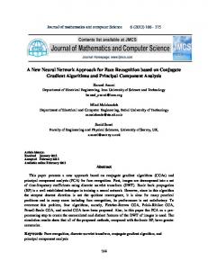
VI. ALGORITHM In this section, a face recognition method by using local database has been suggested and presented. We used an image preprocessing, CMLABP and PCA operations respectively for this procedure. We used real database of images obtained from 100 persons that each person has three images of different situations and positions. Each image has size of 180 x 200 pixels. The detailed procedural steps for face recognition are: 1. Preparing training data set to line up a set of face images as a training set from 1 to N number of faces. In this step, it reforms every 2D image of the training database into 1D column vectors. Then, it relocates 1D column vectors in a row to assemble 2D matrix. 2. Applying illumination normalization. In this study, an easy image preprocessing pipeline is based on [11] that operates effectively for a wide range of visual feature sets. It consists of preprocessing chain, which gives the result as a balanced intensity image. The adopted image preprocessing has been performed through Gamma Correction, Difference of Gaussian (DoG) filtering and Contrast Equalization stages as stated in [11]. The sample face images for our local database and their equivalent preprocessed images are illustrated in Figure 7. The Gamma correction, DOG filtering and contrast equalization values have been set to 0.3, 2 and 0.1 respectively.

Figure 7. Some sample of faces and their equivalent preprocessed images for local database 3. Employing feature extraction by CMLABP. Firstly, the LABP operation is applied using Eq.(8) based on the average gray-values of pixels. In this case, the threshold is employed from the standard deviation value of each pixel. Then, 4 co-occurrence matrices for each LABP image are computed for {[0 1], [-1 1], [-1 0], [-1 -1]} offsets that are resolved as one adjoining pixel in the potential four

‫اﻟﻤﺠﻠﺔ اﻟﻌﺮاﻗﻴﺔ ﻟﻠﻬﻨﺪﺳﺔ اﻟﻜﻬﺮﺑﺎﺋﻴﺔ واﻻﻟﻜﺘﺮوﻧﻴﺔ‬ 2017 ، 1 ‫ اﻟﻌﺪد‬، 13 ‫ﻡﺠﻠﺪ‬ directions. Finally, all co-occurrence matrices and 6 Haralic features are grouped into single feature vector to construct the CMLABP representation. 4. Lastly, the feature dimensionality reduction and recognition operations can be done by PCA method. In this method, the mean value is computed and the deviation of each image from the mean value will be calculated. After that, a step to sort and eliminate eigenvalues is required. Then, eigenvectors of covariance matrix C (eigenfaces) are calculated. They can be recovered from A's Eigenvectors. Recognition is done by Projecting centered image vectors into face space. All centered images are projected into face space by multiplying in eigenface basis. Projected vector of each face will be its equivalent feature vector. Lastly, Euclidean distance between projected test image and the projection of the entire centered training images will be evaluated. If Euclidean distance between a test image and training images is zero, it will be considered as an identified face image. Otherwise, it will be considered as an unidentified face image. Each 2D face image with M × N size can be converted to 1D vector of MN dimension. For instance, face image from ORL database with 112 × 92 size can be converted to a vector of dimension 10,304 or homogeneously a point in a 10,304 dimensional space.

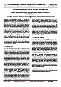
VII. RESULTS Face is a complicated multidimensional image model and expanding a computational model for face recognition is tricky. An additional demanding state is recognition at a distance, when the subject matter is sensed in random circumstances. In this scenario, persons can be distant from the camera or uninformed of the sensors. In these conditions, the challenge comes from these types of awkward users. In the case of the pattern of the subject is obtained with an impartial expression, it is easy for a person who attempts to keep away from being sensed to adjust parts of his or her facial surface by a cheering or openmouthed expression. Likewise, on the growing of a moustache or a beard, or wearing glasses may generate a difficulty in the process of identifying the person. A possible key solution to this difficulty is to make use of just the rigid divisions of the face, most particularly the nose region, for identification. Nevertheless, limiting the input data to such a miniature area indicates that much practical information will be lost, and the large accuracy will be reduced. Image preprocessing (PP), CMLABP and PCA integration method reduce these effects. In this section a methodology for face recognition has been adopted. The main goal of this study is to apply the system (model) for any specified face and recognize it from a big number of stocked up faces with a number of real-time deviations in addition to his/her personal information as in flowchart depicted in Figure 8.

109

Iraq J. Electrical and Electronic Engineering Vol.13 No.1 , 2017

‫اﻟﻤﺠﻠﺔ اﻟﻌﺮاﻗﻴﺔ ﻟﻠﻬﻨﺪﺳﺔ اﻟﻜﻬﺮﺑﺎﺋﻴﺔ واﻻﻟﻜﺘﺮوﻧﻴﺔ‬ 2017 ، 1 ‫ اﻟﻌﺪد‬، 13 ‫ﻡﺠﻠﺪ‬

Figure 9. Face recognitions for different poses and situations The test Image for any person can be captured by using a webcam as in Figure 10. This webcam can be adjusted using GUI display as in Figure 11.The used webcam in this work is HD Pro C920 that offers 1080p resolution. It has very good capturing and video resolution. Also, it has physically powerful features and smooth streaming video.

Figure 8. The flow chart of the proposed face recognition

The integration of PP, CMLABP and PCA methods recognizes the similarity of images for chosen people with high performance. Accordingly, we used chosen input images to compare between them and images from a database by using our algorithm that shows the similar and non-similar images. This method can identify an image in different poses and situations, even in the cases of growing a beard, or wearing glasses or moved eyes or open mouths or even aging as shown in Figure 9.

Figure 10. The adopted webcam for proposed face recognition model

110

Iraq J. Electrical and Electronic Engineering Vol.13 No.1 , 2017

‫اﻟﻤﺠﻠﺔ اﻟﻌﺮاﻗﻴﺔ ﻟﻠﻬﻨﺪﺳﺔ اﻟﻜﻬﺮﺑﺎﺋﻴﺔ واﻻﻟﻜﺘﺮوﻧﻴﺔ‬ 2017 ، 1 ‫ اﻟﻌﺪد‬، 13 ‫ﻡﺠﻠﺪ‬

Figure 11. General GUI display As it can be seen from Figures 12-13, this model will display the person information in the case of face identification. Otherwise, if the input face is new to a database system, in this case his /her information must be entered in database for future use and identification. It must be indicated that the success rate for proposed model is better than 99 % for 100 different person face images with 3 images of each person using a local database. Using higher developed cameras can enhance the recognition rate of the proposed algorithm of this study. Other Persons button in the GUI Matlab model can be used to compare any image from any hard disk (internal or external) or from any external storage memory with the stored images in the database. The proposed technique could be used to detect and check the person information if his/her face details was recorded in the local database.

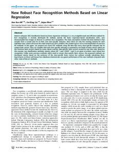
Figure 13. Identification case with citizen information GUI display Finally, the proposed face recognition system has been compared and examined with other reported works in the literature using diverse methods and databases. The applied databases are AR, Yale B, ORL and FERET for this comparison. The sample faces for each applied database are shown in Figure 14 using a scaling factor of 0.1. It is found that the face recognition approach based on the integration of PP, CMLABP and PCA methods of this study has a better recognition rate than reported face recognition systems in [9,10,11,25,27] respectively as it can be observed from Table 1 using the same adopted database and no. of training images in these reported works. Also, it can be utilized as an active tool to discover the cases of forgery and enhance crime investigations. Up to 700 training images, the execution time for our proposed method is within 10 seconds for different applied databases.

Figure 14. The applied databases in this study: (a) ORL; (b) Yale; (c) AR; (d) FERET. Figure 12. Non-identification case with citizen information GUI display

111

Iraq J. Electrical and Electronic Engineering Vol.13 No.1 , 2017

‫اﻟﻤﺠﻠﺔ اﻟﻌﺮاﻗﻴﺔ ﻟﻠﻬﻨﺪﺳﺔ اﻟﻜﻬﺮﺑﺎﺋﻴﺔ واﻻﻟﻜﺘﺮوﻧﻴﺔ‬ 2017 ، 1 ‫ اﻟﻌﺪد‬، 13 ‫ﻡﺠﻠﺪ‬

Table 1 Comparison of the proposed face recognition with [9], [10], [11] [25] and [27] using same applied database and the number of training images Algorithms/Parameter

Database Type

Method

No. of Training images 700

Max Recognition Percentage(%) 94.7, 98.1

Max Recognition Percentage of Our Work(%) 99.4, 99.9

Face recognition technique reported in [9]

AR, Yale B databases

SRC

Face recognition technique reported in [10] Face recognition technique reported in [11] Face recognition technique reported in [11] Face recognition technique reported in [25] Face recognition technique reported in [27]

AR LBP+SRC database ORL PP + LBP database PP+LBP+PCA ORL database ORL Eigen Faces database

700

96

99.4

300

94.66

99.667

300

98.78

`99.667

190

97.5

99.47

ORL, Yale B, FERET databases

400

99.4, 97.5, 98

99.75, 99.5, 99.25

Common Eigen values

REFERENCES

VIII. CONCLUSION 1. In this research article, a well-organized face recognition system has been proposed. This system has hardware and software parts. The hardware component consists of a camera, whereas the software part has face-recognition algorithm program using Matlab simulator. The adopted identification processes with local features provide very good and rapid classification for face recognition. It has a very useful system for face recognition with an identification rate more than 99%. The success is attributed to the integration of image preprocessing, CMLABP and PCA methods. The performance of the matching procedure can be used to display the personal information such as (name, surname, birth date, etc.) in the case of face match or record his/ her information for future use in the case of non-matching by comparing the captured image with local database images. This can be used for forgery or crimes investigations. The recognition rate of the proposed face recognition technique is higher than reported face recognition systems in [9,10,11, 25, 27] using same applied database and the number of training images.

2.

3.

4.

5.

6.

7.

112

W. Y. Zhao, R. Chellappa, P. J. Phillips, and A. Rosenfeld, “ Face Recognition: A Literature Survey,” ACM Computing Surveys, vol.34, no. 4, pp. 399–485, 2003. A. K. Jain, R. Ross, and S. Prabhakar, “ An Introduction to Biometric Recognition,” IEEE Transaction on Circuits and Systems for Video Technology, vol.14, no. 1, pp. 84-92, 2004. K. Dharavath, F. A. Talukdar, and R. H. Laskar , “ Improving Face Recognition Rate with Image Preprocessing,” Indian Journal of Science and Technology, vol.7, no. 8, pp.1170–1175, 2014. J. Meng, and Y.Yang, “Symmetrical Two Dimensional PCA with Image Measures in Face Recognition,” International Journal of Advanced Robotic Systems, vol.9, pp.238-248, 2012. C. Zhang and W.-S. Chen , “A Novel Fisher Criterion Based Approach for Face Recognition,” Proceedings of IEEE International Conference on Wavelet Analysis and Pattern Recognition, Tianjin, pp. 27-31, 2013. S. Nazari, and M. S. Moin , “Face Recognition Using Global and Local Gabor Features,” Proceedings of 21st IEEE Iranian Conference on Electrical Engineering, Mashhad, pp. 1-4, 2013. A. Suruliandi , K. Meena, and R. Reena-Rose , “Local Binary Pattern and Its Derivatives for Face

Iraq J. Electrical and Electronic Engineering Vol.13 No.1 , 2017

8.

9.

10.

11.

12.

13.

14.

15.

‫اﻟﻤﺠﻠﺔ اﻟﻌﺮاﻗﻴﺔ ﻟﻠﻬﻨﺪﺳﺔ اﻟﻜﻬﺮﺑﺎﺋﻴﺔ واﻻﻟﻜﺘﺮوﻧﻴﺔ‬ 2017 ، 1 ‫ اﻟﻌﺪد‬، 13 ‫ﻡﺠﻠﺪ‬

Recognition,” IET Computer Vision, vol. 6, no. 5, pp. 480 – 488, 2012. A. H. Bishak, Z. Ghandriz, and T. Taheri , “Face Recognition using Co-occurrence Matrix of Local Average Binary Pattern, ”Journal of Selected Areas in Telecommunications, April Edition, pp.15-19, 2012. J. Wright, A. Ganesh, A. Yang, and Y. Ma, “Robust Face Recognition via Sparse Representation, ” IEEE Transactions on Pattern Analysis and Machine Intelligence, vol. 31, no. 2, pp. 210-227, 2009. R. Min, and J.-L. Dugelay, “Improved Combination of LBP and Sparse Representation Based Classification (SRC) for Face Recognition, ” Proceedings of IEEE International Conference on Multimedia and Expo (ICME), Barcelona, pp.16, 2011. P. S. Sonar, and P. K. Ajmera , “Face Recognition using Local Texture Descriptor, ” International Journal of Engineering Research and Technology, vol. 3, no. 4, pp. 642-646, 2014. Z.-Q. Zhao, D.S. Huang, and B.-Y. Sun, “ Human Face Recognition Based on Multiple Features Using Neural Networks Committee, ” Pattern Recognition Letters, vol. 25, no. 12, pp. 13511358, 2004. Y.-F. Hou, Z.-L. Sun, Y.-W. Chong, and C.-H. Zheng, “ Low-Rank and Eigenface Based Sparse Representation for Face Recognition, ” PLoS ONE Journal , vol. 9. no.10, pp. 1-14, 2014. E. Dong, Y. Fu, and J. Tong , “Face Recognition by PCA and Improved LBP Fusion Algorithm, ” Applied Mechanics and Materials, vol. 734, pp. 562-567, 2015. Z. Mahmood, T. Ali, and S. U. Khan, “Effects of Pose and Image Resolution on Automatic Face Recognition, ” IET Biometrics, vol. 5, no.2, pp. 111–119, 2016.

20. 21.

22.

23.

24.

25.

26.

27.

16. J. Rehab, and F. Hardalac , “Retinal Blood Vessel Segmentation with Neural Network by Using Gray-Level Co-Occurrence Matrix-Based Features, ” Journal of Medical Systems, vol. 38, no. 85, pp. 1-12, 2014. 17. K. Nissim, and E. Harel, A Texture Based Approach to Defect Analysis of Grapefruits. Georgia Institute of Technology, CS7321 Winter, 1997. 18. R. Haralick, K. Shanmugam, and I. Dinstein , “Textural Features for Image Classification, ” IEEE Transactions on Systems, Man, and Cybernetics, vol.3, no.6, pp. 610-621, 1973. 19. N. Otsu , “A Threshold Selection Method from Gray- Level Histogram, ” IEEE Transactions on

113

Systems, Man, and Cybernetics, vol.9, no.1, pp. 62-66, 1979. R. C. Gonzalez, and R. E. Woods, Digital Image Processing, Prentice Hall, New Jersey, 2008. R. Shams, and R. A. Kennedy, “Efficient Histogram Algorithms for NVIDIA CUDA Compatible Devices, ”Proceedings of International Conference on Signal Processing and Communications Systems, pp. 418–422, 2007. T. Ojala, M. Pietikainen, and D. Harwood , “A Comparative Study of Texture Measures with Classification Based on Feature Distributions, ” Pattern Recognition, vol. 29, no.1, pp. 51–59, 1996. T. Ojala, M. Pietikainen, and T. Maenpaa, “Multiresolution Gray-Scale and Rotation Invariant Texture Classification with Local Binary Patterns, ” IEEE Transactions on Pattern Analysis and Machine Intelligence, vol.24, no.7, pp. 971–987, 2002. M. Turk, and A. Pentland, “Eigenfaces for Recognition , ”Journal of Cognitive Neuroscience vol. 3, no.1, pp.71-86, 1991. M. Slavkovic, and D. Jevtic, “ Face Recognition Using Eigenface Approach, ” Serbian Journal of Electrical Engineering, vol.9, no.1, pp. 121-130, 2012. H. Zhou, Face Detection and Recognition, Biometrics From Fiction to Practice, Pan Stanford Publishing, Singapore, 2013. V. H. Gaidhane, Y. V. Hote, and V. Singh, “ An Efficient Approach for Face Recognition Based on Common Eigenvalues, ” Pattern Recognition, vol.47, no.5, pp. 1869-1879, 2014.