graph model set captures the temporal characteristics of the video frames by adapting the ..... Computer Vision and Image Understanding 91 (2003) 214–245. 9.
Face Recognition in Videos Using Adaptive Graph Appearance Models Gayathri Mahalingam and Chandra Kambhamettu Video/Image Modeling and Synthesis (VIMS) Lab. Department of Computer and Information Sciences, University of Delaware, Newark, DE, USA
Abstract. In this paper, we present a novel graph, sub-graph and supergraph based face representation which captures the facial shape changes and deformations caused due to pose changes and use it in the construction of an adaptive appearance model. This work is an extension of our previous work proposed in [1]. A sub-graph and super-graph is extracted for each pair of training graphs of an individual and added to the graph model set and used in the construction of appearance model. The spatial properties of the feature points are effectively captured using the graph model set. The adaptive graph appearance model constructed using the graph model set captures the temporal characteristics of the video frames by adapting the model with the results of recognition from each frame during the testing stage. The graph model set and the adaptive appearance model are used in the two stage matching process, and are updated with the sub-graphs and super-graphs constructed using the graph of the previous frame and the training graphs of an individual. The results indicate that the performance of the system is improved by using sub-graphs and super-graphs in the appearance model.
1
Introduction
Face recognition has long been an active area of research, and numerous algorithms have been proposed over the years. For more than a decade, active research work has been done on face recognition from still images or from videos of a scene [2]. A detailed survey of existing algorithms on video-based face recognition can be found in [3] and [4]. The face recognition algorithms developed during the past decades can be classified into two categories: holistic approaches and local feature based approaches. The major holistic approaches that were developed are Principal Component Analysis (PCA) [5], combined Principal Component Analysis and Linear Discriminant Analysis (PCA+LDA) [6], and Bayesian Intra-personal/Extra-personal Classifier (BIC) [7]. Chellapa et al. [8] proposed an approach in which a Bayesian classifier is used for capturing the temporal information from a video sequence and the posterior distribution is computed using sequential importance sampling. As for the local feature based approaches, Manjunath and Chellapa [9] proposed a feature based approach in which features are derived from the intensity data without assuming
2
Gayathri Mahalingam and Chandra Kambhamettu
any knowledge of the face structure. Topological graphs are used to represent relations between features, and the faces are recognized by matching the graphs. Fazl Ersi and Zelek [10] proposed a feature based approach in which Gabor histograms are generated using the feature points of the face image and are used to identify the face images by comparing the Gabor histograms using a similarity metric. Wiskott et al. [11] proposed a feature based approach in which the face is represented as a graph with the features as the nodes and each feature described using a Gabor jet. A similar framework was proposed by Fazl-Ersi et al. [12] in which the graphs were generated by triangulating the feature points. Video-based face recognition has the advantage of using the temporal information from each frame of the video sequence. Zhou et al. [13] proposed a probabilistic approach in which the face motion is modeled as a joint distribution, whose marginal distribution is estimated and used for recognition. Li [14] used the temporal information to model the face from the video sequence as a surface in a subspace and performed recognition by matching the surfaces. Kim et al. [15] fused pose-discriminant and person-discriminant features by modeling a Hidden Markov Model (HMM) over the duration of a video sequence. Stallkamp et al. [16] used K-nearest neighbor model and Gaussian mixture model (GMM) for classification purposes. Liu and Chen [17] proposed an adaptive HMM to model the face images. Lee et al. [18] represented each individual by a low dimensional appearance manifold in the ambient image space. Park and Jain [19] used a 3D model of the face to estimate the pose of the face in each frame and then matching is performed by extracting the frontal pose from the 3D model. In this paper, we propose a novel adaptive graph based approach that uses graphs, sub-graphs, and super-graphs for spatially representing the faces for face recognition in a image-to-video scenario. The graphs, sub-graphs and supergraphs are constructed using the facial feature points as vertices which are labeled by their feature descriptors. An adaptive probabilistic graph appearance model is built for each subject, which captures the temporal information. Adaptive matching is performed using the probabilistic model in the first stage and a graph matching procedure in the second stage. The appropriate appearance model is updated with the results of recognition from the previous frame of the video sequence, and the associated graph model set is updated with the subgraphs and super-graphs generated using the graph of the previous frame and the model graphs.
2
Face Image Representation
In this section, we describe our approach in representing the face images. In our approach, the face image is represented by a graph which is constructed using the facial feature points as vertices. The vertices are labeled by their corresponding feature descriptors which are extracted using the Local Binary Pattern (LBP) [20], [21]. Every face is distinguished not by the properties of individual features, but by the contextual relative location and comparative appearance of
Face Recognition in Videos Using AGAM
3
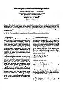
these features. Hence, it is important to identify those features that are conceptually common in every face such as eye corners, nose, mouth, etc. The feature points are extracted by using a similar approach as [1], where the authors extract the features points using a modified Local Feature Analysis (LFA) [22] which constructs kernels that spatially represent a pixel in the image. A subset of kernels are extracted that correspond to discriminative facial features using Fisher scores. Figure 1 shows the feature points extracted from the image and a frame of the video sequences. The images are ordered according to their resolution from high to low.
Fig. 1. First 150 Feature points extracted from the training image (first pair of images) and the testing video frames (second & third pair of images)
2.1
Feature Description with Local Binary Pattern
A feature descriptor is constructed for each feature point extracted from an image using Local Binary Pattern (LBP). The original LBP operator proposed by Ojala et al. [20] labels the pixels of an image by thresholding the n × n neighborhood of each pixel with the value of the center pixel, and considering the result value as a binary number. The histogram of the labels of the pixels is used as a texture descriptor. The LBP operator with P sampling points on a circular neighborhood of radius R is given by,
LBPP,R =
P −1 X
s(gp − gc )2p .
(1)
p=0
where � s(x) =
1 if x ≥ 0 0 if x < 0
(2)
The LBP operators with at most two bitwise transitions from 0 to 1 or vice versa were called as uniform patterns by Ojala et al. which reduced the dimension u2 of LBP significantly. In our experiments, we use LBP8,2 which represents an uniform LBP operator with 8 sampling points in a radius of 2 within a window of 5 × 5 around the pixel which give a 59 element vector.
4
3
Gayathri Mahalingam and Chandra Kambhamettu
Adaptive Graph Appearance Model
An adaptive appearance model is constructed for each subject using the set of feature points and their descriptors from all the images of the subject. The appearance of a graph is another important distinctive property and is described using the feature descriptors of the vertices of the graph. In our approach, we construct a graph appearance model by modeling the joint probability distribution of the appearance of the vertices of the graphs of an individual. The probabilistic appearance model is constructed using the feature descriptors from all the images of a subject which makes it easy to adapt to the changes in the size of the training data. The model can easily be adapted to the changes in the training set as it is constructed using the feature descriptors. The adaptation is performed at the matching stage where the result of recognition from each frame is adapted to the appropriate appearance model. Given N individual and M training face images, the algorithm to learn the model is described as follows: 1. Initialize N empty model sets. 2. For each individual i with Mi images a. For each image Iij , (j th image of the ith individual) ∗ Extract feature points and corresponding feature descriptors (subsection 2.1). ∗ Construct image graphs (subsection 3.1) and add it to the ith model set. b. For each pair of graphs in the ith model set ∗ Extract the feature points for sub-graph and super-graph (subsection 3.2). ∗ Construct the sub-graph and super-graph using the extracted feature points (subsection 3.2) and add it to the ith model set. c. Construct the appearance model for the ith individual using the ith model set. The appearance model denoted as Φn is constructed by estimating the joint probability distribution of the appearance of the graphs which is modeled using Gaussian Mixture Model (GMM) [23]. GMMs can efficiently represent heterogeneous data and capture dominant patterns in the data using Gaussian components. Mathematically, a GMM is defined as: P (F |Θ) =
K X
wi N (X|µi , σi )
(3)
i=1
where N (X|µi , σi ) = K
1 √
σi 2π
exp−
(X−µi )2 2σ 2
(4)
and Θ = wi , µi , σi2 i=1 are the parameters of the model, which includes the weight wi , the mean µi , and variance σi2 of the K Gaussian components. In order to maximize the likelihood function P (F |Θ), the model parameters are re-estimated using the Expectation-Maximization (EM) technique [24]. For more details about the EM algorithm see [24].
Face Recognition in Videos Using AGAM
3.1
5
Image Graph Construction
The most distinctive property of a graph is its geometry, which is determined by the way the vertices of the graph are arranged spatially. Graph geometry plays an important role in discriminating the graphs of different face images. In our approach, the graph geometry is defined by constructing a graph with constraints imposed on the length of the edges between a vertex and its neighbors. We propose a graph generating procedure that generates a unique graph with the given set of vertices for each face image. At each iteration, vertices and edges are added to the graph in a Breadth-first search manner and considering a spatial neighborhood distance for each vertex. This generates a unique graph given a set of feature points. The following proof illustrates the uniqueness property of the graph generated. Theorem 1. Given a set of vertices V , the graph generation procedure generates a unique graph G(V, E). Proof. Proof by contradiction. Let there be two graphs G1 (V, E1 ) and G2 (V, E2 ) generated by the graph generation procedure, such that G1 6= G2 . In other words, E1 6= E2 . Without loss of generality, let us assume that there exists an edge e ∈ E1 which connects two vertices u and v, where u, v ∈ V , and e 6∈ E2 . This implies that the Euclidean distance between u and v is greater than the threshold, and hence e 6∈ E1 as well. Hence, E1 = E2 ⇒ G1 = G2 . Hence the proof. 3.2
Common sub-graph and super-graph
The graph representation effectively represents the inherent shape changes of a face and also provides a simple and powerful matching technique. Including the shape changes and the facial deformations caused by pose changes in the model improves the recognition rate. In our approach, we capture these shape changes due to change in pose of the face by constructing a common sub-graph and super-graph using the set of graphs of an individual. The common sub-graph and super-graph are defined in our system as follows; Definition 1. Given two graphs G1 and G2 , the sub-graph H of G1 and G2 is defined as H = {v|v ∈ G1 ∩ G2 , 3 cos(f1 (v), f2 (v)) ≈ 1, f1 (v) ∈ G1 , f2 (v) ∈ G2 }
(5)
where v is the vertex, e is the edge, and f (v) is the feature descriptor of v. The sub-graph includes those vertices that have spatial similarity and vertex similarity in G1 and G2 . Definition 2. Given two graphs G1 and G2 , the super-graph H of G1 and G2 is defined as H = {v|v ∈ G1 ∪ G2 } (6) where v is the vertex, e is the edge, and f (v) is the feature descriptor of v.
6
Gayathri Mahalingam and Chandra Kambhamettu
The sub-graphs and super-graphs are constructed for each pair of graphs of the images of a subject using a similar approach to construct the graph of an image. The sub-graph and super-graph essentially capture the craniofacial shape changes and the facial deformations due to various poses of the face.
4
Adaptive Matching and Recognition
We use a two stage adaptive matching procedure to match every frame of the video with the trained models and graphs. The first stage of matching involves the computation of a Maximum a Posterior probability using the test graph G(V, E, F ) with vertex set V and set of feature vectors F and is given by, Pk = max P (G|Φn ). n
(7)
where Pk is the MAP probability of G belonging to model set k. The MAP solution is used to prune the search space for the second stage of matching in which we use a simple deterministic algorithm that uses cosine similarity measure and spatial similarity constraints to compare the test graph with the training graphs. The appropriate GMM is adapted by the result of recognition and is used for matching subsequent frames. The recognition result is considered correct if the difference between the highest score and the second highest score is greater than a threshold. This measure of correctness is based on the idea proposed by Lowe [25], that reliable matching requires the best match to be significantly better than the second best match. The appropriate model set and the GMM is updated with the result of recognition from each frame. The update involves adding the graph of the frame to the model set, along with the sub-graphs and super-graphs generated using the graph of the frame and the graphs in the model set. The entire matching procedure is given as follows; 1. For each frame f in the video sequence a. Construct the image graph G using the extracted feature points and their descriptors. b. Compute the MAP solution for G belonging to each appearance model and select k model sets (10% in our experiments) with highest probability. c. Compute similarity scores between G and the graphs from k model sets using cosine similarity measure. d. Update the appropriate GMM and the model set with G using the likelihood score and similarity scores. 2. Select the individual with the maximum number of votes from all the frames. An iterative procedure is used to find the similarity between graphs. Given two graphs G and H with |H| ≤ |G|, we use spatial similarity (spatial location of a vertex in H and G) and vertex similarity (vertices with similar feature descriptors) to match H with a subgraph of G that maximizes the similarity score. At each iteration, vertex u ∈ H is compared with v ∈ G such that u
Face Recognition in Videos Using AGAM
7
and v have high spatial and vertex similarity. The procedure is repeated with neighbors of u and v. The spatial constraint imposed on the vertices reduces the number of vertex comparisons and allows for faster computation.
5
Experiments
In order to validate the robustness of the proposed technique, we used the UTD database [26]. The UTD database consists of a series of close and moderate range, videos of 315 subjects and also their high resolution images in various poses. The neutral expression close range videos and the parallel gait videos were used in our experiments. The high resolution images of each subject were used as training set. Figure 2 shows sample video frames of both the close-range and moderate-range videos from the UTD database. The preprocessing steps include extracting the face region and resizing it to 72 × 60 pixels. We extracted 150 feature points from each image and their corresponding feature descriptors were computed using 5 × 5 window around each point. The dimension of the feature vectors are reduced using PCA from 59 to 20 retaining 80% of the non-zero eigenvalues. Graphs including sub-graphs and super-graphs are generated for the images of each individual. The maximum spatial neighborhood distance of each vertex was set to 30 pixels. A GMM with 10 Gaussian components is constructed for each individual using the set of graphs. K-means clustering is used for initializing the GMM.
(a) Sample video frames from UTD (b) Sample video frames from UTD dataset in close-range database in moderate-range Fig. 2. Sample video frames from the UTD video datasets
During the testing stage, we randomly selected a set of frames from the videos of a subject. A graph is generated for each frame after preprocessing the frame. The likelihood scores are computed for the test graph and the GMMs and the training graphs are matched with the test graph to produce similarity scores, and the appropriate GMM is updated using the similarity and likelihood scores. The threshold is determined by the average of the difference in likelihood scores and similarity scores between each class of data. Though the threshold value is data dependent, the average proves to be an optimum value. The performance of the algorithm is compared with video-based recognition algorithm in [17] (denoted as HMM) which handles video-to-video based recognition. In addition to this, we compare the performance by considering the effects of temporal information and spatial information individually and when combined. We
8
Gayathri Mahalingam and Chandra Kambhamettu Table 1. Comparison of the error rates with different algorithms HMM AGMM Graphs AGMM+Graphs UTD Database (close-range) 24.3% 24.1% UTD Database (moderate-range) 31.2% 31.2%
21.2% 16.1% 26.8% 19.4%
denote the above two approaches as AGMM and Graphs respectively, and the proposed approach as AGMM+Graphs. The results are tabulated in the Table 1. Figure 3 shows the Cumulative Match Characteristic curve obtained for various algorithms (AGMM+Graphs, AGMM and HMM).
(a) CMC curve for close-range videos (b) CMC curve for moderate-range of UTD database videos of UTD database Fig. 3. Cumulative Match Characteristic curves for close-range and moderate-range videos
A few observations were made from the error rates and the CMC curves. The first observation is that the recognition performance is improved by the spatial representation using the sub-graph, and super-graph representations. It is evident from the results that the account of spatial and temporal information together improves the performance of the system in case of matching high resolution images with that of low resolution videos. This observation can be made from the error rates of the HMM approach and our approach. The inclusion of spatial information in addition to the temporal information provided by the HMM or AGMM improves the performance of the system. The second observation is that the close-range videos of the UTD database has lower error rates than the moderate-range videos. This is due to the fact that the frame of the video sequence mostly contains the face region thus gathering more details of the facial features than the moderate-range videos. The third observation is that the adaptive appearance model along with the update to the graph model sets improves the performance significantly from our previous work [1]. This is due to adding graphs, sub-graphs and super-graphs to the model set and the appearance model that is spatially similar to those generated for each frame of the individual. Also, the chance of updating the incorrect appearance model is low
Face Recognition in Videos Using AGAM
9
due to the abundant spatial information available from the graphs. The fourth observation is that the performance of the system is affected by the amount of training data given for each individual. The lack of sufficient training images of a subject affect the performance of the system. This eventually leads us to the conclusion that the system’s performance can be improved in the case of videovideo based face recognition where the training set is a set of videos which has more number of frames with the wealth of spatial and temporal information. The effect of various parameters on the performance was also tested. From our experiments, we observed that the parameters do not significantly affect the performance of the system. For example, increasing the maximum Euclidean distance between two vertices of a graph to a value greater than the width or length of the image will have no effect as this does not change the spatial neighborhood of a vertex in the graph. Hence, a lower threshold value of half the value of the width of face region was set to ensure a connected graph. The Gaussian components of a GMM represented heterogeneous data of the training set which are basically various facial features (e.g. eyes, nose, mouth, etc.). Hence, the 10 Gaussian components were sufficient to represent the heterogeneous facial features.
6
Conclusion
In this paper, we proposed a graph based face representation for face recognition from videos. The spatial characteristics are captured by constructing graphs for each face image and extracting the common sub-graphs and super-graphs from the set of graphs of each subject. An adaptive graph appearance model is generated that incorporates the temporal characteristics of the video sequence. A modified LFA and LBP were used to extract the feature points and feature descriptors, respectively. A two stage adaptive matching procedure that exploits the spatial and temporal characteristics is proposed for efficient matching. The experimental results show that graph based representation is robust and gives better performance. As a future work, we would like to test the system on videovideo based face recognition and other standard databases with benchmarks.
References 1. Mahalingam, G., Kambhamettu, C.: Video based face recognition using graph matching. The 10th Asian Conference on Computer Vision (2010) 2. Chellapa, R., Wilson, C.L., Sirohey, S.: Human and machine recognition of faces: a survey. Proceedings of the IEEE 83 (1995) 705–741 3. Wang, H., Wang, Y., Cao, Y.: Video-based face recognition: A survey. World Academy of Science, Engineering and Technology 60 (2009) 4. Zhao, W., Chellappa, R., Phillips, P.J., Rosenfeld, A.: Face recognition: A literature survey (2000) 5. Turk, M., Pentland, A.: Eigenfaces for recognition. Journal of Cognitive Neuroscience 3 (1991) 71–86
10
Gayathri Mahalingam and Chandra Kambhamettu
6. Etemad, K., Chellapa, R.: Discriminant analysis for recognition of human face images. Journal of the Optical Society of America 14 (1997) 1724–1733 7. Moghaddam, B., Nastar, C., Pentland, A.: Bayesian face recognition using deformable intensity surfaces. In Proceedings of Computer Vision and Pattern Recognition (1996) 638–645 8. Zhou, S., Krueger, V., Chellappa, R.: Probabilistic recognition of human faces from video. Computer Vision and Image Understanding 91 (2003) 214–245 9. Manjunath, B.S., Chellapa, R., Malsburg, C.: A feature based approach to face recognition (1992) 10. Ersi, E.F., Zelek, J.S.: Local feature matching for face recognition. In Proceedings of the 3rd Canadian Conference on Computer and Robot Vision (2006) 11. Wiskott, L., Fellous, J.M., N.Kruger, Malsburg, C.V.D.: Face recognition by elastic bunch graph matching. IEEE Trans. on Pattern Analysis and Machine Intelligence 19 (1997) 775–779 12. Ersi, E.F., Zelek, J.S., Tsotsos, J.K.: Robust face recognition through local graph matching. Journal of Multimedia (2007) 31–37 13. Zhou, S., Krueger, V., Chellapa, R.: Face recognition from video: A condensation approach. In Proc. of fifth IEEE Internation Conference on Automatic Face and Gesture Recognition (2002) 221–228 14. Li, Y.: Dynamic face models: construction and applications. Ph.D. Thesis, University of London (2001) 15. Kim, M., Kumar, S., Pavlovic, V., Rowley, H.A.: Face tracking and recognition with visual constraints in real-world videos. CVPR (2008) 16. Stallkamp, J., Ekenel, H.K.: Video-based face recognition on real-world data (2007) 17. Liu, X., Chen, T.: Video-based face recognition using adaptive hidden markov models. CVPR (2003) 18. Lee, K.C., Ho, J., Yang, M.H., Kriegman, D.: Visual tracking and recognition using probabilistic appearance manifolds. Computer Vision and Image Understanding 99 (2005) 303–331 19. Park, U., Jain, A.K.: 3d model-based face recognition in video (2007) 20. Ojala, T., Pietikainen, M., Harwood, D.: A comparative study of texture measures with classification based on feature distributions. Pattern Recognition (1996) 51–59 21. Ojala, T., Pietikainen, M., Maenpaa, T.: A generalized local binary pattern operator for multiresolution gray scale and rotation invariant texture classification. Second International Conference on advances in Pattern Recognition, Rio de Janeiro, Brazil (2001) 397–406 22. Penev, P., Atick, J.: Local feature analysis: A general statistical theory for object representation. Network: Computation in Neural Systems 7 (1996) 477–500 23. McLachlam, J., Peel, D.: Finite mixture models (2000) 24. Redner, R.A., Walker, H.F.: Mixture densities, maximum likelihood and the em algorithm. SIAM Review 26 (1984) 195–239 25. Lowe, D.G.: Distinctive image features from scale-invariant keypoints. International Journal of Computer Vision 60 (2004) 91–110 26. O’Toole, A., Harms, J., Hurst, S.L., Pappas, S.R., Abdi, H.: A video database of moving faces and people. IEEE Transactions on Pattern Analysis and Machine Intelligence 27 (2005) 812–816