Face Recognition in Complex Background - Semantic Scholar

International Journal of Smart Home Vol. 9, No. 10, (2015), pp. 47-62 http://dx.doi.org/10.14257/ijsh.2015.9.10.06

Face Recognition in Complex Background: Developmental Network and Synapse Maintenance 1

Dongshu Wang and 2Lei Liu

1

School of Electrical Engineering, Zhengzhou University, Zhengzhou, China, 450001 [email protected] 2Department of Financial Research, People’s Bank of China, Zhengzhou SubBranch, Zhengzhou, China, 450040 [email protected] Abstract As an important sub-field in computer vision and pattern recognition, face recognition has important theoretical and practical application. It is a very complicated problem which is often affected by variations in illumination condition, head pose, facial emotions, glasses, beards, and so on. 108 face images of 27 learned objects (appearances) from complex backgrounds in BioID face database are efficiently recognized with the developmental network (DN) - a biologically inspired framework with the emergent representation. But the DN has no adaptive receptive field for an object with a curved contour. Leaked-in background pixels can lead to problems when different objects look similar. This paper introduces another biologically inspired mechanism - synapse maintenance to achieve the object recognition. Synapse maintenance can automatically decide which synapse should be removed, kept or partial removed, thus it can weaken the complex background, strengthen the face features, reduce the bad influence of the complex background on the face recognition. Experimental results show that DN with the synapse maintenance can effectively recognize faces with complicated backgrounds and the recognition rate is over 95%. Keywords: Developmental Network, Face Recognition, Emergent Representation, Synapse Maintenance, Recognition Rate

1. Introduction With the development of image processing, artificial intelligence, computer vision, statistics learning, cognitive theory and psychology, as a main component of the biometric method, two dimensional face recognition has become an important technique in national safety and public security, due to its universality, uniqueness and non-invasion [1]. It has been widely used in social security, financial, custom, civil aviation and military security, etc. Two dimensional face recognition uses the face images to identify the subjects through abstracting face recognition features. For its high academic value and important applications, since the early 70's of the last century, face recognition has been a topic of intense research in the recent past and has drawn the attention of researchers in fields from security, psychology, and image processing, to computer vision [2]. As summarized in [3], past work on face recognition has been focused on digital images taken in highly constrained environments. Strong assumptions are used to make the task more tractable. For example, there is usually just one front-view face in the center of the image, the head is upright, the background is clean, no occlusion of faces exists, no

ISSN: 1975-4094 IJSH Copyright ⓒ 2015 SERSC

International Journal of Smart Home Vol. 9, No. 10, (2015)

glasses are worn, and so on. The existence and locations of human faces in these images are known a priori, so there is little need to detect and locate faces [4]. But most of the face recognition systems are used in non-ideal environments. With the variations of facial expressions, glasses, beards, gestures, poses and lighting, etc, the system performance will be affected inevitably. Especially, under the interference from noises or complex backgrounds, the recognition rate will be decreased greatly. So the two dimensional face recognition in complex backgrounds is an very challenging problem. In real applications, the subject contours are arbitrary but the receptive fields are usually regular (such as square) in the image scanning. Therefore, leak of pixels of backgrounds in the receptive field is very difficult to be avoided which may bring disturbance [5]. But in the competitive self-organizing, among the neurons who have almost the same receptive field, the modes resulting from foreground objects emerge relatively more often than those of backgrounds. In addition, neurons whose bottom-up weights match a foreground object pretty well, usually obtain top-down attention coming from a motor area more likely to be a winner. Though their default receptive fields can not match the contour of a foreground object well, among the situations during the neuron fires, the standard deviation of pixels from the foreground object are usually smaller than that of pixels in backgrounds. Based on this theory, this paper introduces a new biologically inspired mechanism - synapse maintenance - to determine concise input fields based on the statistics, without manual setting what feature each neuron detects. In the remainder of the paper, related works about 2D face recognition in complex background and synapse maintenance are introduced in Section II. Theories about developmental network and synapse maintenance are presented in Section III. Experiments procedure is depicted and results are analyzed in Section IV. Concluding remarks are provided in Section V.

2. Related Work 2.1. 2D Face Recognition in Complex Background The real face recognition research originated in 1965, in that year, Chan and Bledsoe presented a technical report about the face recognition in Panoramic Research Inc, which brought the first step of face intelligent recognition [6]. Now, the main face recognition algorithms originated from the early researches of many experts. In order to enhance the robustness of the face recognition system, many scholars have attempted various approaches and have obtained some excellent achievements. Huang [7] proposed the NMF method based on alpha divergence for face recognition under noise interferences or complex backgrounds. This method used the alpha divergence to measure the distance, and many iterative factorization expressions can be gotten by different parameter values in the corresponding NMF expressions. The difference degree is computed at each step of iteration to determine the optimal parameter at the next step, so as to ensure that NMF converges to the global optimum and improve the precision of face recognition. Chen et al. [8] presented a real-time face detection and recognition system for mobile robots based on videos with a complex background. Face detection part is composed of an Adaboost algorithm and a skin color model to detect faces against a complex background rapidly and efficiently. The interesting objects in the video were first detected by the Adaboost algorithm, and then the skin color model was adopted to select the parts that may not be skin areas from the information detected by the Adaboost algorithm. An embedded hidden Markov model was proposed to recognize the faces detected. In [9], an efficient face recognition system based on Haar wavelet and Block Independent Component Analysis (BICA) algorithm was presented. The adaptive boosting classifier is trained with Haar features to classify and detect faces, and the BICA

48

Copyright ⓒ 2015 SERSC

International Journal of Smart Home Vol. 9, No. 10, (2015)

algorithm is used to recognize the detected face. This system is able to detect the face in the field of view of camera in real time and testify the object's identity if the images of this object have already been trained by the system. This system is able to detect the face even with slight occlusions and under varying lighting and it can improve the recognition rate obviously. Of course, it goes without saying that, beside these aforementioned researches, there are still a lot of issues designing robust and reliable face recognition algorithms in complex background. For example, the subspace methods have had successful applications in face recognition, which include principal component analysis (PCA) [10], Kernel PCA [11], wavelet transform [12], Eigen face [13, 14], Fisher's linear discriminant analysis (FLDA) [15, 16], Kernel LDA [17], independent component analysis (ICA) [18], Kernel ICA [19], Kernel DCV [20], non-negative matrix factorization (NMF) [21]. Furthermore, other algorithms, such as support vector machine (SVM) [22, 23], Markov random field [24], etc, have also been presented to enhance the accuracy of face recognition in complex background. However, up to now, face recognition in complex background is still a very complicated problem and big challenge. The general face recognition approaches include feature extraction from different face databases and feature classification. One of the drawbacks of these techniques is that they don't use human brain's super abilities to recognize the face. Our aim is to apply the achievements of the proposed models based on human vision system. Neurologists' researches show that, processes in vision path and cortexare is composed of feed-forward computations and receiving feedback from higher layers. Instead of implementing in one step, the recognition task in human is performed in several feedforward and recursive steps and what is recognized in each step, is employed in order to model correspondence in the next steps [25]. In this work, we deal with emergent representations of the face images in unsupervised learning in the internal neurons of the developmental network (DN). By internal, it means that all the neurons inside a brain are not directly supervised by the external environment --- outside the brain skull. The motor port (denoted as Z area below) is partially open, roughly corresponding to the peripheral nervous system. We are interested in what such internal neurons represent while they are not directly supervised by the external environment. 2.2. Developmental Network Developmental network is the basis of a series of where-What networks, whose 9th version, namely, the latest version, appeared in [26]. The simplest version of a developmental network has three areas, the sensory area X , the internal area Y , and the motor area Z , with an example in Fig. 1. The internal area Y as a "bridge" to connect its two "banks"- the sensory area X and the motor area Z , depicted mathematically as X Y Z (1) Where denotes two one-way connections. The DN algorithm is as follows. Input areas: X and Z , Output areas: X and Z . The dimension and representation of X and Y areas are hand designed based on the sensors and effectors of the robotic agent or biologically regulated by the genome. Y Is skullclosed inside the brain, not directly accessible by the external world after the birth (1) At time t = 0, for each area A in { X , Y , Z }, initialize its adaptive part N  V , G  and the response vector r , where V contains all the synaptic weight vectors and G stores all the neuronal ages.

Copyright ⓒ 2015 SERSC

49

International Journal of Smart Home Vol. 9, No. 10, (2015)

Figure 1. The Architecture of the Developmental Network It contains top-down connections from Z to Y for context represented by the motor area. It contains top-down connections from Y to X for sensory prediction. Pink areas are human taught. Yellow areas are autonomously generated (emergent and developed). Although the foreground and background areas are static here, they change dynamically. (2) At time t = 1, 2, , for each area A in { X , Y , Z }, do the following two steps repeatedly forever: (a) Every area A computes using area function f (2)  r, N   f  b, t, N    (b) For each area A in { X , Y , Z }, A replaces: N  N and r  r . If X is a sensory area, x  X is always supervised and then it does not need any synaptic vector. The z  Z is supervised only when the teacher chooses to. Otherwise, z gives (predicts) motor output. Next, we describe the area function f . Each neuron in area A has a weight vector v   vb , vt  , corresponding to the area input  b, t  , if both bottom-up part and top-down part are applicable to the area. Otherwise, the missing part of the two should be removed from the notation. Its pre-action energy is the sum of two normalized inner product: v t v b (3) r (vt , t , vb , b)  t   b   v p || vt || || t || || vb || || b || Where v the unit is vector of the normalized synaptic vector v   vt , vb  and p is the

unit vector of the normalized synaptic vector p  (t , b) . To simulate lateral inhibition (winner takes all) within each area A, only top- k winners fire and update. Considering k = 1, the winner neuron j is identified by: j  arg max r(vbi , b, vti , t ) (4) 1i  c

Where c is the neuron number in the area A. The area dynamically scale top- k winners so that the top-k responses with values in [0, 1]. For k = 1, only the single winner fires with response value y j  1 and all other neurons in A do not fire. The response value y j approximates the probability for p to

50

Copyright ⓒ 2015 SERSC

International Journal of Smart Home Vol. 9, No. 10, (2015)

fall into the Voronoi region of it’s v j where the "nearness" is r(vt , t, vb , b) . All the connections in a DN are learned incrementally based on Hebbian learning co-firing of the pre-synaptic activity p and the post-synaptic activity y of the firing neuron. Here, we consider area Y as the example, as other area learns in a similar way. If the pre-synaptic end and the post-synaptic end fire together, the synaptic vector of the neuron has a synapse gain yp . Other non-firing neurons do not modify their memory. When a neuron j fires, its weight is updated by a Hebbian-like mechanism: (5) v j  1 (n j )v j  2 (n j ) y j p Where 2 (n j )

is the learning rate and 1 (n j )

the retention rate and

1 (n j )  2 (n j )  1 . The simplest formula of 2 (n j ) is 1 n j , which gives the recursive computation of the sample mean of input p : vj 

1 nj

nj

 p t  i 1

i

(6)

Where ti is the firing time of the neuron, the age of the winner neuron j is incremented n j  1  n j . A component in the gain vector y j p is zero if the corresponding component in p is zero. Each component in v j so incrementally computed is the estimated probability for the pre-synaptic neuron to fire under the condition that the postsynaptic neuron fires. 2.3. Synapse Maintenance In order to solve the problem of leaked-in background pixels in the 2D face recognition, synapse maintenance [5, 26, 27] was presented to automatically determine and regulate the receptive field of a neuron. The network intends to keep some synapses which have better matches and remove other synapses. With the synapse maintenance, the network can improve its performance significantly. But the above mentioned work only considers the synapse maintenance in the bottom-up input from Y area. At the birth time of the Developmental Network, neurons in Y connect with both X and Z . Neurons in Y integrate the bottom-up and top-down inputs, connecting motors which represent simple and intuitive concepts with X area. For complicated concepts, the internal signal in Z area must be transmitted by the Y neurons. If we further explore the external world, we can find that the Y area is divided into different regions in terms of certain connections. Neuroscience experiments have demonstrated that there exist the early processing area and later processing area in human vision system. However, up to now, human beings still do not know the principle and mechanism of vision cortex division well. Therefore, humans have not established a reasonable model to solve this problem in neuroscience or artificial intelligence field. Cross-domain synapse maintenance [28] adopted in this paper maybe a feasible way of emergence in Y with the computer simulation. Through the cross-domain synapse maintenance, the neurons in Y can dynamically remove some synapses which connect with irrelevant inputs. In real environments, due to the foreground object's arbitrary contours, changing backgrounds in the receptive fields of Y neurons will affect the recognition results as described in section 3.2. Naturally, we will generate an idea like this: if the network can discriminate the foreground and the background or automatically summarize the object contours, the irrelevant components (i.e., the backgrounds) in the receptive fields of the Y neurons can be cut to reduce the backgrounds interference in the object recognition. Synapse maintenance mechanism is exactly designed to implement this thought (i.e., cutting the irrelevant components, while keeping those relevant ones) by computing the standard deviation of each pixel in different images.

Copyright ⓒ 2015 SERSC

51

International Journal of Smart Home Vol. 9, No. 10, (2015)

Each neuron in Y area has three input domains: bottom-up b , lateral l and top-down t [26]. In complicated tasks such as the face recognition in complex background, the discrimination of neurons in Y means that some domains with irrelative input should be deleted totally. Trimming and keeping of a synapse from a certain domain relies on the correlation of weight and input which is determined by the standard deviation ratio to the expected deviation among all the domains. It is important to know that synapse maintenance works among all the three input domains and integrates the second order statistical characteristics of these inputs to modulate the contributions of three domains in Y area. Based on the aforementioned researches, this paper uses the developmental network with the emergent inferring ability to recognize the 108 images of 27 persons in BioID face database. To testify the recognition effect, in initializing the weights from X layer to Y layer, two methods are adopted: random initialization and using the input images' weights as the initial weights. Furthermore, with the two initializing methods, we studied the different recognition accuracy under different neurons of Y layer and different competing neurons (different k in top-k) in Y layer, to demonstrate the performance of DN in the face images recognition in complex background.

3. Related Concepts and Algorithm 3.1. Receptive Fields Perceived by Y Neurons In initial stage, neurons in Y connect with both X and Z . Some neurons in Y whose synapses with X are scheduled regularly and tightly have fixed and intensive receptive fields, so they can detect stable features from input image [5]. These neurons in Y have the local receptive fields from the retina shown as Fig. 2. Assume the receptive field is a  a , the neuron  i, j  perceives the region R  x, y  in the input image ( i  x  i  a  1 , j  y  j  a  1 ), where the coordinate  i, j  denotes the location of the neuron on the two-dimensional plane and similarly the coordinate  x, y  represents the location of the pixel on the input image.

rea aa n i t Re

be l lo a t i cip Oc

Figure 2. The Illustration of the Receptive Fields of Neurons In Y area, on the contrary, these neurons whose synapses with X are scheduled loosely and randomly, have sparse and big receptive fields, therefore their inputs from X area are random. With the cross-domain synapse maintenance mechanism, the latter neurons will gradually trimthe synapses connecting with X and handle signals from motor areas especially.

52

Copyright ⓒ 2015 SERSC

International Journal of Smart Home Vol. 9, No. 10, (2015)

3.2. Foreground and Background In this work, "foreground" means the objects to be recognized with arbitrary contours, on the contrary, "background" is the left part in the whole image. In the default receptive field of an occipital lobe neuron, there are two kinds of pixels: foreground pixels and background pixels. Pre-action energy of each neuron is calculated from both the foreground match and the background match. Though the contribution from foreground pixels can afford a high pre-action value when the foreground object is correct, the contribution from background pixels often gives a random value. Therefore, we can not guarantee that the winner neuron usually brings the right recognition [5]. In this work, a new biological mechanism, synapse maintenance, is introduced into the DN to reduce the background interference automatically through removing some synapses. 3.3. Theory of the Synapse Maintenance Synapse maintenance is seemed to be carried out by each neuron in the brain. Each neuron which is generated from neurogenesis (mitosis), can autonomously decide where to connect in the neural network. But in the Developmental Network (DN), each neuron does not have a pre-selected feature to detect, thus the role of each neuron is dynamically determined through its interactions with other neurons-known as the process of autonomous development [28]. A neuron is assumed to have an initial input vector p which is defined by all its spines where synapses locate. The neuron will cut all the synapse components in p which is irrelevant to its postsynaptic firing (i.e., cluttered backgrounds in vision), but at the same time, it can minimize the cutting of those relevant ones (i.e., a foreground object). This cutting is based on statistical calculation of the match, between the pre-synaptic activities and the synaptic conductance (weight). The well-known synaptic factors include acetylcholine, agrin, astrocytes, neuroligins. SynCAM and their co-workers [29] have demonstrated that partial blockage of the acetylcholine receptor (AChR) can cause the retraction of corresponding pre-synaptic terminals. It is believed that ACh can denote expected uncertainty, in other words, "this neuron predicts this pre-synaptic line pretty well." Assume that the input to a neuron is P  ( p1, p2,..., pd ) and its synaptic weight vector is

V （v1 , v2 ,..., vd）. Because each synapse locates on its spine, so it is necessary to indicate that this synaptic weight vector is the comprehensive effect of both the spines and the synapses. Acetylcholine (ACh) originates from the basal forebrain in the brain, and it can signal the expected uncertainty [28]. Here we will study how to neuromorphically measures the expected uncertainty. When top- k neurons fire with value y , its synapse denotes the mean of the pre-synaptic activities vi

 i  E  ypi the neuron fires]

(7)

Using amnesic average, the standard deviation of the match between vi and pi is a measure of expected uncertainty for each synapse i : (8)  i  E | vi  pi || the neuron fires is the expected uncertainty for each synapse, modeled by ACh. Mathematically,  i is the expected standard deviation of the match of the synapse i . In calculating the expected uncertainty, it must begin with a constant value and wait till all the weights of the neuron have good estimates of wi . Assume that  i (n) is  i at firing age n . When n  n0 , each synapse begins with the standard deviation of uniform distribution in   ,   . Then, the synapse i begins with normal incremental average. At

Copyright ⓒ 2015 SERSC

53

International Journal of Smart Home Vol. 9, No. 10, (2015)

last, a constant asymptotic learning rate is used to make the standard deviation be continuously plastic. The expression for synapse deviation is computed incrementally as follows:   / 12 n  n0 (9)  i ( n)   n  n0 1 (n) i (n  1)   2 (n) vi  pi Where

1   (n) , （ (10)  1   2 ( n) 1 n） n Where nij is the age of the neuron, or the firing times of the neuron.  (nij ) is the

（  2 n）

amnesic factor, its expression is:  0 if   (nij )  c  (ni j  t1 ) (t2  t1 ) if  c  (ni  t ) r if j 2 

nij  t1 t1  nij  t2 t2  nij

(11)

And in this work, we set the waiting latency n0  6 , to wait until synapse weights become good estimates through the first n0 updates. That is to say, synapse maintenance works after the same neuron is fired for 6 times. Each neuron should dynamically determine which synapse should keep active and which one should be removed relying on the goodness of the match. The expected goodness of the match is denoted by the expected uncertainty. The expected synaptic deviation among all the synapses of a neuron is defined by the following formula: 1 d (12)  ( n)    i ( n) d i 1 Where we suppose that each neuron only has a single section of input b , l , t . 3.4. Cross-Domain Synapse Maintenance In the DN model, each neuron in Y has three domains of input: bottom-up b , lateral l and top-down t , and all the inputs are excitatory. The inhibitory input is simulated by top- k competition. The bottom-up domain b is X area and lateral domain l is Y area. It should be pointed out that each pre-synaptic activity has been normalized into the range [0, 1] where 0 means not firing and 1 means firing. Therefore, the  ij from the j th neuron in the i -th domain needs to be compared. This comparison is needed as an entire domain. However, because the dimensions are different in different domains, it is necessary to note that a low-dimensional domain plays a considerable role as a high-dimensional domain. Therefore, the expected synaptic deviation in Eq.(12) should be modified to the following multi-domain version:  1 s ( n )   i di ( n )  (n)   ij (n)  (13)    c(n) i 1  di (0) i 1  where s(n) is the number of domains including 1-D domain, d i the dimension of domain i ,  i the percentage of energy for domain i , d (n) the current dimension of the input source p after one or more domains have probably been cut, and c(n) is to make sure that the sum of all weights is one: s(n)

c( n )  

i

(14) di (n) di (0) Though we use only di (0) and i (0) to set the initial weights of each domain, this expression permits one or more domains (or sub-domains) to be removed completely, for i 1

54

Copyright ⓒ 2015 SERSC

International Journal of Smart Home Vol. 9, No. 10, (2015)

example, the bottom-up, lateral, Z domains have energy percentages 1/3, 1/3 and 1/3, respectively, to sum to 100%. Let wi (n ) 

i

c(n)d i (0) We can obtain the expected synaptic deviation as follows:

(15)

 di ( n )   (n)   wi (n)    ij (n)  (16) i 1  j 1  The above expression means that in a domain with fewer synapses, each synapse has more voice in vote for the  (n) . The neuronal samples of relative ratios are defined as novelty transmitters Norepinephrine (NE):  (n) (17) rij ( n )  ij  (n) The cross-domain synaptogenic factor which uses three linear segments is defined as follows: 1 rij (n)   s   (18) f ( rij (n ))  (  b  rij (n)) / (  b   s )  s  rij (n)   b  0  b  ri (n)  We should cut these synapses whose  (n) are relatively large. If the relative ratios of deviation in a domain i are all higher than  b , all synapses in this domain should be removed. Based on the domain weighted distribution of rij in different domains, we can s(n)

achieve  s and  b for synapse connecting with X and Z , separately. 3.5. Synapse Trimming Synapse trimming can be considered as the maintenance of spine synapse combination. Trimming of weights vector V （v1 , v2 ,..., vd）can be defined (19) f ( ri (n))  vi  vi

i  1,2,

, d . In an analogy way, trimming the input vector P   p1 , p2 , , pd 

can be defined as follows: f (ri (n))  pi  pi

(20)

Where p   b, l , t  .Then the trimmed response's calculating should be modified accordingly, it follows that the synapse factor can dynamically determine whether the corresponding synapse can provide a full supply, no supply, or in between. Using trimming, the area function that includes synaptic maintenance is as follows. Algorithm 1 (area function with synaptic maintenance). Do the following steps: 1. Every neuron trims it’s p   b, l , t  and V （vb , vl , vt）respectively, using Eqs. (19) and (20). 2. Every neuron performs  -mean normalization for each of b , l and t , respectively, of the input vector p   b, l , t  , where   12  and   1 256 , unless the input vector is a scalar. 3. Every neuron computes the pre-action potential using trimmed inner product:  b  l  t vb  vl  vt  r ( p, v )       (21)        e  b  e  vb    e  l  e  vl    e  t  e  vt        

Copyright ⓒ 2015 SERSC

55

International Journal of Smart Home Vol. 9, No. 10, (2015)

where   0 ,   0 ,   0 with       1 and e( x)  x   where    12 . The default values for  ,  ,  are  =  =  =1/3. 4. Conduct top-k competition for all neurons in the Y layer. 5. Only the winner neurons conduct Hebbian learning to update their synaptic weight vectors using their normalized firing values and their own trimmed input vectors. Other neurons do not fire. 6. Only the winner neurons update  i for each synapse, update their  , and advance their ages. Other neurons do not update. 7. Only the winner neurons update the synaptogenetic factors f . Other neurons do not update.

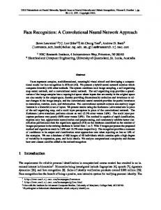
4. Face Recognition with DN In this study, we use images of 27 persons in BioID face dataset to be the experimental samples, each person (subject) representing a different type to be recognized, to testify the performance of DN on the 2D face recognition. The BioID database contains 115 male and female gray-scale images. Each person has 5 different gray-scale images. Images of the individuals have been taken with varying lighting condition, facial expression (open/close eyes, smiling/not smiling), facial details (glasses/no glasses, mustache/no mustache) and different backgrounds. The images are manually cropped and re-scaled to a resolution of 384  286, with bit grey levels. Six images of each subject are used for training and four for testing, giving a total of 168 training and 108 test images. The examples of BioID database is illustrated in Figure 3.

Figure 3. Samples of the BioID Face Database 4.1. Experiment Design 4.1.1. Establish the Network: In DN, X layer takes the image pixels as the input, i.e., 384  286 grey values, so the input from X layer to Y layer is a matrix of (384  286,1); neuron number of Y layer is adjustable, first, we adopt 10  10 neurons (later, 8  8, 6  6, 5  5 are also considered); neuron number of Z layer is 27, i.e., 27 faces to be recognized. Thus, the input from Z to Y is a matrix of (27, 1) 4.1.2. Weights and Ages Initialization: Weights from X layer to Y layer, Y layer to

56

Copyright ⓒ 2015 SERSC

International Journal of Smart Home Vol. 9, No. 10, (2015)

Z layer, and Z layer to Y layer, are all initialized randomly. Neurons age of Y and Z layer are all initialized with 1.

4.2. Experiment Procedure In training phase, read the images from the training set directly and input them to X layer. Pre-action energy (response) of Y neurons can be calculated with expression (3) and the neuron whose energy is the largest will be fired. For this fired neuron, its weights will be updated by the expression (5), where 2 (n j )  1  age  1 , where age is the neuron's current age. If a neuron is fired, its age will be added 1 each time. Those neurons who do not fire keep their weights and ages unchangeable. Using this response matrix to be the input of Y layer to Z layer, we can calculate the responses of the Z layer neurons. Input from Y to Z is 100*1 matrix, in this matrix, element value corresponding to the fired neuron of Y is set 1 and others is set 0. Similarly, in Z layer, neuron whose energy is the largest will be fired. This fired neuron corresponds the network inferring results, in other words, subject corresponding to the input image. After connecting with the fired neuron in Y layer, the fired neuron in Z layer updates its weight in the same way as the neuron in Y layer. In testing phase, the DN is "frozen". That is to say, structure of the DN is determinate and the weights can not be updated. X Layer input the testing images, then the responses of the neurons in Y layer are calculated, the output of the neuron whose pre-action energy is the largest will be set 1 and other neurons 0. Using this response matrix to be the input of Y layer to Z layer, the pre-action energies of the neurons of Z layer can be calculated. The person corresponding to the neuron with the largest pre-action energy is the final recognition result of the DN. 4.3. Experiment Results In order to evaluate the effect of DN on the face recognition, this work compares the recognition speed and rate, with and without the synapse maintenance mechanism. 4.3.1. DN without the Synapse Maintenance: This experiment aims to investigate the effect of the DN on the face recognition with the different Y neuron number and different top- k ( k denotes the number of the fired neuron), without the synapse maintenance. Initializing the weights from X layer to Y layer randomly, and the inputs of X layer are the grey values of the current input image. This method can retain the individuality efficiently in seeking the generality. After the first image enters the DN, in order to prevent the following images superposing on the first one, thus affecting the recognition accuracy, a suitable threshold is used. That is to say, after inputting an image each time, the pre-action energies of Y neurons are calculated. If the energy is larger than the threshold, the corresponding neuron is fired. Otherwise, a new neuron of Y layer is distributed. This method occupied bigger store space (i.e., more Y layer neuron number). Repeating the former procedure, we can achieve the results shown in table 1 Table 1. Recognition Rate Comparison among Different Cases without the Synapse Maintenance 12  12 10  10 88 66 55

Copyright ⓒ 2015 SERSC

k 1

k 2

k 3

1.0000 1.0000 0.8719 0.8241 0.6574

0.9537 0.8889 0.8611 0.5648 0.5000

0.9444 0.8426 0.8148 0.5463 0.4573

57

International Journal of Smart Home Vol. 9, No. 10, (2015)

From Table 1, we can see that when the Y layer has more neurons, the recognition accuracy is above the 95%, with the decreasing of the neuron number of Y layer, the recognition accuracy also decreases. When the neuron number of Y layer (e.g., 5  5) is smaller than that of the subjects to be recognized (i.e., 27), the recognition accuracy decreases significantly. The reason is that even in the case of k =1, the Y layer has no sufficient neurons to assign to each class to be recognized. Under the condition of the same neuron number of Y layer, with the increasing of top- k , the accuracy decreases a little. It results from the cross phenomenon produced by increasing Y layer neuron number assigned to the same subject. 4.3.2. DN with the Synapse Maintenance: This part is designed to study the effect of the DN on the face recognition with the different Y neuron number and top- k , considering the synapse maintenance function. Experiment procedure is the same as the former experiment. The corresponding results are presented in Table 2. Table 2. Recognition Rate Comparison among Different Cases with the Synapse Maintenance 12  12 10  10 88 66 55

k 1

k 2

k 3

1.0000 1.0000 0.9074 0.8333 0.6944

0.8889 0.7963 0.8519 0.4815 0.3426

0.7963 0.8333 0.5833 0.3426 0.2130

Based on the table 2, we can see that when the neuron number of Y layer is larger than the recognized image number 27, and if there is only one neuron of Y to fire each time (i.e., top-1 is used), the recognition accuracy is 95%. Similarly, when the neuron number of Y layer (e.g., 5  5) is smaller than the subject classes to be recognized (i.e., 27), the recognition accuracy decreases obviously. 4.3.3. Performance Comparison: To compare the recognition performance of the DN with and without synapse maintenance, the recognition rates in different epochs are investigated and shown in Table 3. Table 3. Recognition Rate Comparison of the DN with and without the Synapse Maintenance Epochs DN without synapse maintenance DN with synapse maintenance

1

2

3

4

5

6

7

8

0.9341

0.9388

0.9437

0.9778

0.9907

0.9982

1.0000

1.0000

0.9331

0.9489

0.9828

1.0000

1.0000

1.0000

1.0000

1.0000

To present the difference vividly, we display the performance difference in Figure 4. From table 3 and Figure 4, it is obvious that the final recognition rate is almost the same, but because of the synapse maintenance removing the irrelevant components and keeping the relevant components, the recognition speed of the DN with the synapse maintenance is faster than that of the DN without the synapse maintenance. If the Y layer has more neurons (to simulate the brain's complex neural network more efficiently), the speed advantage of the DN with the synapse maintenance will be more obvious

58

Copyright ⓒ 2015 SERSC

Recognition rate (%)

International Journal of Smart Home Vol. 9, No. 10, (2015)

100 99 98 97 96 95 94 93 92 91

with synapse maintenance without synapse maintenance 0

1

2

3

4 Epochs

5

6

7

8

Figure 4. Recognition Performance Comparison of the DN with and without Synapse Maintenance 4.4. Specific Experiment Results and Analysis In this part, we adopt the following specific parameters to testify the recognition performance: Y layer neurons 10  10, k =1, t1 =6, t2 =9, c =1.5. After the training, we can get the following figures.

Figure 5. Weights from X Layer to Y Layer From Figure 5, we can see that in the training phase, 55 of the 100 neurons are fired to recognize the 27 different faces.

Copyright ⓒ 2015 SERSC

59

International Journal of Smart Home Vol. 9, No. 10, (2015)

Figure 6. Synapse Deviation  n of the Y Neurons In Figure 6, the white contours are the images to be recognized, corresponding to the images in Figure 5. The black parts in the images are the weakened backgrounds. The black sub-images on the right side are the neurons not fired. Their initial values of the synapse deviation  n are 1 256 12 , and they are normalized in plotting, as a result, their pixel values are all 0 after conversion, thus shown as the black. The initial value of the synapse factor is set 1, and it begins to work only after neuron age reaches t1 . There are 27 subjects to be recognized, so there are 27 neurons which use the synapse maintenance. Figure 6 and Figure 7 testify the correctness of the DN in recognizing the 2D face images indirectly.

Figure 7. SYNAPTOGENIC Factor f of the Y Neurons

5. Conclusion This work uses the DN to recognize the face images of 27 subjects from the complex

60

Copyright ⓒ 2015 SERSC

International Journal of Smart Home Vol. 9, No. 10, (2015)

background. To overcome the drawback of the DN and improve the recognition speed, a biological inspired mechanism -- synapse maintenance, is introduced to the DN, to automatically remove the irrelevant inputs and keeping the relevant ones. This work compared the performance between the DN with and without the synapse maintenance, and the inherent reasons are analyzed. Experimentally, we demonstrate that the DN can achieve a faster recognition rate with the synapse maintenance.

Acknowledgements The authors want to thank the help from Professor Juyang Weng with Department of Computer Science and Engineering, Michigan State University, MI, USA, and Qian Guo with Department of Electronic Engineering, Fudan University, and Shanghai, China.

References [1] Y. Ming, “Research on 3D face recognition based on invariant features”, PHd Thesis of Beijing Jiaoting University, (2012) pp. 1-3. [2] S. H. Lin, “An Introduction to Face recognition Technology, Informing Science Special Issue on multimedia informing technologies”, Part 2, vol. 3, no. 1, (2000), pp. 1-7. [3] A. Samal and P. A. Iyengar, “Automatic recognition and analysis of human faces and facial expressions”, A survey, Pattern Recognition, vol. 25, no. 1, (1992), pp. 65-77. [4] H. Wang and S. Chang, “Editors, A Highly Efficient System for Automatic Face Region Detection in MPEG Video”, IEEE TCSVT, Special Issue on Multimedia Technology, Systems, and Applications (MA018), (2011), pp. 1-26. [5] Y. Wang, X. Wu and J. Weng, “Editors, Synapse maintenance in the where-what network, International Joint Conference on Neural Network (IJCNN)”, (2011) July 31-August 5, San Jose, CA. [6] H. Chan and W. W. Bledsoe, “A man-machine facial recognition system: some preliminary results”, Panoramic Research Inc., Cal, (1965). [7] A. Huang, “Editors, NMF Face Recognition Method Based on Alpha Divergence”, Proceedings of the International Conference on Information Engineering and Applications (IEA), Lecture Notes in Electrical Engineering, (2012) October 26-28, Chongqing, China. [8] S. Chen, T. Zhang, C. Zhang and Y. Cheng, “A real-time face detection and recognition system for a mobile robot in a complex background”, Artificial Life and Robotics, no. 15, (2010), pp. 439-443. [9] V. Vaidehi, A. A. Fathima, T. M. Treesa, M. Rajasekar, P. Balamurali, M. G. Chandra and Editors, “An Efficient Face Detection and Recognition System”, Proceedings of the International Multi Conference of Engineers and Computer Scientists (IMECS), (2011) March 16-18, HongKong, China. [10] G. P. Teja, S. Ravi and Editors, “Face Recognition Using Subspaces Techniques”, 2012 International Conference on Recent Trends in Information Technology (ICRTIT), (2012) April 19-21, Chennai, India. [11] Y. Zhang and C. Liu, “Face Recognition using Kernel Principal Component Analysis and Genetic Algorithms”, Neural Network for Signal Processing, (2002), pp. 337-343. [12] B. L. Zhang and Y. Guo, “Face recognition by wavelet domain associative memory”, Intelligent Multimedia, Video and Speech Processing, (2001), pp. 481-485. [13] M. Turk and A. Pentland, “Eigen-faces for recognition”, Journal of Cognitive Neuroscience, vol. 3, no. 1, (1991), pp. 71-86. [14] Y. Hou, W. Pei, Y. Chong and C. Zheng, “Editors, Eigenface-Based Sparse Representation for Face Recognition”, 2013 International Conference on Intelligent Computing (ICIC2013), (2013) July 28-31, Nanning, China. [15] K. Etemad and R. Chellappa, “Discriminant analysis for recognition of human face images”, Journal of the Optical Society of America, vol. 14, no. 8, (1997), pp. 1724-1733. [16] A. Bansal, K. Meht and S. Arora, “Editors, Face Recognition Using PCA and LDA Algorithms”, 2012 Second International Conference on Advanced Computing and Communication Technologies, (2012) May 14-16, Rohtak, Haryana. [17] M. H. Yang, “Editors, Kernel Eigenfaces vs. Kernel Fisherfaces, face recognition using kernel methods”, Proceedings of international conference on automatic face and gesture recognition, (2002) May 20-21, Washington DC, USA. [18] M. S. Bartlett, J. R. Movellan and T. J. Sejnowski, “Face recognition by independent component analysis”, IEEE Trans Neural Networks, vol. 13, no. 6, (2002), pp. 1450-1464. [19] T. Martiriggiano, M. Leo, T. Dorazio and A. Distante, “Face Recognition by Kernel Independent Component Analysis, Innovations in Applied Artificial Intelligence, Lecture Notes in Computer Science”, vol. 3353, (2005), pp. 55-58. [20] Y. H. He, L. Zhao and C. R. Zou, “Editors, Kernel discriminative common vectors for face recognition”, Proceedings of international conference on machine learning and cybernetics, (2005) August 18-21, Guangzhou, China.

Copyright ⓒ 2015 SERSC

61

International Journal of Smart Home Vol. 9, No. 10, (2015)

[21] C. J. Lin, “Projected gradient methods for nonnegative matrix factorization”, Neural Computation, no. 19, (2007), pp. 2756-2779. [22] W. Wang, X. Sun and S. Karungaru, “Editors, Face Recognition: An algorithm Using Wavelet decomposition and Support Vector Machines”, 2012 international symposium on opt mechatronic technologies (ISOT), (2012) Oct 29-31, Paris, France. [23] S. Valuvanathorn, “Editors, Multi-Feature Face Recognition based on PSO-SVM, 2012 Tenth International Conference on ICT and Knowledge Engineering”, (2012) November 21-23, Bangkok, Thailand. [24] H. T. Ho and R. Chellappa, “Pose-Invariant Face Recognition Using Markov Random Fields”, IEEE Transactions on image processing, vol. 22, no. 4, (2013), pp. 1573-1584. [25] J. A. Jalali and J. Amiryan, “Editors, A Novel Bidirectional Neural Network for Face Recognition”, 2012 2nd International eConference on Computer and Knowledge Engineering (ICCKE), (2012) October 1819, Mashhad, Iran. [26] Q. Guo, X. Wu and J. Weng, “WWN-9: Cross-domain synaptic maintenance and its application to object groups recognition”, 2014 International Joint Conference on Neural Networks, (2014) July 6-11, Beijing, China. [27] Y. Wang, X. Wu and J. Weng, “Editors, Brain-like learning directly from dynamic cluttered natural video”, International Conference on Brain-Mind (ICBM), (2012) July 14-15, East Lansing, MI [28] J. Weng, Editor, Natural and Artificial Intelligence: Introduction to computational brain-mind, BMI press, Okemos, Michigan, USA (2012). [29] C. M. McCann, Q. T. Nguyen, H. S. Neto and J. W. Lichtman, “Rapid synapse elimination after postsynaptic protein synthesis inhibition in vivo”, The Journal of Neuroscience, vol. 27, no. 22, (2007), pp. 6064-6067.

Authors Dongshu Wang, received his Bachelor’s degree in Mechanical Manufacture Technique and Equipment in1996, Masters degree in Mechanical Manufacture and Automation in 2002, and PhD in Control Theory and Control Engineering in 2006 from Northeastern University, China. His research domain is autonomous mental development and artificial intelligence. Currently, he is an Associate Professor in School of Electrical Engineering, Zhengzhou University, Zhengzhou, China.

Lei Liu, received her Bachelor degree in Accounting in 1997 from Northeastern University, Master degree in Accounting in 2001 from Zhongnan University of Economics and Law, PhD in Quantitative Economics in 2008 from Huazhong University of Science and Technology, Her research domain is financial risk control and intelligent computation. Currently, she is a research associate professor in the Department of Financial Research, People's Bank of China, Zhengzhou Central Sub-Branch, Zhengzhou, China.

62

Copyright ⓒ 2015 SERSC