Facilitating Neural Dynamics for Delay Compensation and Prediction in Evolutionary Neural Networks Heejin Lim
Yoonsuck Choe
Department of Computer Science Texas A&M University, 3112 TAMU College Station, TX 77843-3112
Department of Computer Science Texas A&M University, 3112 TAMU College Station, TX 77843-3112
[email protected]
[email protected]
ABSTRACT
1.
Delay in the nervous system is a serious issue for an organism that needs to act in real time. For example, during the time a signal travels from a peripheral sensor to the central nervous system, a moving object in the environment can cover a significant distance which can lead to critical errors in the effect of the corresponding motor output. This paper proposes that facilitating synapses which show a dynamic sensitivity to the changing input may play an important role in compensating for neural delays, through extrapolation. The idea was tested in a modified 2D pole-balancing problem which included sensory delays. Within this domain, we tested the behavior of recurrent neural networks with facilitatory neural dynamics trained via neuroevolution. Analysis of the performance and the evolved network parameters showed that, under various forms of delay, networks utilizing extrapolatory dynamics are at a significant competitive advantage compared to networks without such dynamics. In sum, facilitatory (or extrapolatory) dynamics can be used to compensate for delay at a single-neuron level, thus allowing a developing nervous system to stay in touch with the present environmental state.
Delay is an unavoidable problem for a living organism, which has physical limits in the speed of signal transmission within its system. Such a delay can cause serious problems as shown in Fig. 1. During the time a signal travels from a peripheral sensor (such as the photoreceptor) to the central nervous system (e.g. the visual cortex), a moving object in the environment can cover a significant distance which can lead to critical errors in the motor output which was based on that input. For example, the neural latency between visual stimulus onset and the motor output can be no less than 100 ms up to a couple of hundred milliseconds [31]: An object moving at 40 mph can cover about 9 m in 500 ms (Fig. 1b). However, the problem can be overcome if the central nervous system can take into account the neural transmission delay (∆t) and generate action based on the estimated current state S(t+∆t) rather than that in its periphery at time t (S(t), Fig. 1c). Such a compensatory mechanism can be built into a system at birth, but such a fixed solution is not feasible because the organism grows in size during development, resulting in gradually increased delay. For example, consider that the axons are stretched to become longer during growth. How can the developing nervous system cope with such a problem? This is the main question investigated in this paper. Psychophysical experiments such as flash-lag effect (FLE) showed that extrapolation can take place in the nervous system. In visual flash-lag effect, the position of a moving object is perceived to be ahead of a briefly flashed object when they are in fact physically co-localized at the time of the flash [25, 34, 4, 18]. One interesting hypothesis arising from the flash-lag effect is that of motion extrapolation: Extrapolation of state information over time can compensate for delay, and flash-lag effect may be caused by such a mechanism [25, 10, 7]. According to the motion extrapolation model, a moving object’s location is extrapolated so that the perceived location of the object at a given instant is the same as the object’s actual location in the environment at that precise moment, despite the delay. The perceptual effect demonstrated in the flash-lag effect indicates that the human nervous system performs extrapolation to align precisely its internal perceptual state with the environmental state. The question that arises at this point is, how can such an extrapolatory mechanism be implemented in the nervous system? It is possible that recurrently connected networks
General Terms Experimentation, Algorithm, Performance
Categories and Subject Descriptors I.2.6 [Artificial Intelligence]: Learning
Keywords Neural delay, delay compensation, facilitating synapses, extrapolation, pole balancing, evolutionary neural networks
Permission to make digital or hard copies of all or part of this work for personal or classroom use is granted without fee provided that copies are not made or distributed for profit or commercial advantage and that copies bear this notice and the full citation on the first page. To copy otherwise, to republish, to post on servers or to redistribute to lists, requires prior specific permission and/or a fee. GECCO’06, July 8–12, 2006, Seattle, Washington, USA. Copyright 2006 ACM 1-59593-186-4/06/0007 ...$5.00.
167
INTRODUCTION
Peripheral Sensors
S(t)
Peripheral Sensors
Central Nervous System
Central Nervous System
t+∆tt
St
Environmental State
Environmental State
St
St ?
A(S(t)) A(S t)
S(t)
S(t)
tt+ + ∆t t
tt
(a) Initial state (time t)
(b) No extrap. (time t + ∆t)
Peripheral Sensors
Central Nervous System
t+∆tt
2. A(S(t+ A(S t + t ) ∆t))
FACILITATING AND DECAYING NEURAL DYNAMICS
There are several different ways in which temporal information can be processed in a neural network. For example, decay and delay have been used as learnable parameters in biologically motivated artificial neural networks for temporal pattern processing [32]. Several computational models also include neural delay and decay as an integral part of their design [8, 3]. However, in these works, the focus was more on utilizing delay for a particular functional purpose such as sound localization [12], rather than recognizing neural transmission delay as a problem to be solved in itself. We introduce delay in the arrival of sensory input to hidden neurons so that each internal neuron generates its activation value based on the outdated input data (i.e. put the network in the same condition as the nervous system, which has neural delay). Recent neurophysiological experiments have uncovered neural mechanisms that can potentially contribute to delay compensation. Researchers have shown that different dynamics exist at the synapse, as found in depressing or facilitating synapses [22]. In these synapses, the activation level (the membrane potential) of the postsynaptic neuron is not only based on the immediate input at a particular instant but is also dependent on the rate of change in the activation level in the near past. These synapses have been studied to find the relationship between synaptic dynamics and temporal information processing [9, 11, 29]. However, to our knowledge, these mechanisms have not yet been investigated in relation to delay compensation. Such a mode of activation found in these experiments is quite different from conventional artificial neural networks (ANNs) where the activation level of the neurons are solely determined by the current input and the connection weight values. For example, in conventional ANNs, activation value Xi (t) of a neuron i at time t is defined as follows: X Xi (t) = g wij Xj (t) , (1)
Environmental State
St+
Our overall results suggest that neurons with facilitatory activity can effectively compensate for neural delays, thus allowing the central nervous system to be in touch with the environment in the present, not in the past. In the following, first, the facilitating neural dynamics will be derived (Sec. 2). Next, the modified 2D pole-balancing problem will be outlined (Sec. 3) and the results from the modified cart-pole balancing problem will be presented and analyzed (Sec. 4). Finally, discussion and conclusion will be presented (Sec. 5 and 6).
t
S(t+∆ t)
t +t+∆t
(c) With extrap. (time t + ∆t) Figure 1: Interaction between agent and environment under internal delay. (a) The state S(t) of a moving object (solid circle) in the environment is received at the sensors in an agent (e.g., an animal) at time t. (b) Delay (∆t) in the central nervous system causes error in the resulting action A(S(t)), if state S(t) is not extrapolated. (c) No error if the action is based on a predicted (or extrapolated) state of the object, S(t + ∆t).
of neurons in the brain can provide such a function, since recurrence makes available the history of previous activations [6]. However, such historical data alone may not be sufficient to effectively compensate for neural delay since the evolving dynamics of the network may not be fast enough. Our hypothesis is that for fast extrapolation, the mechanism has to be implemented at a single neuron level. In this paper, we developed a recurrent neural network with facilitatory neural dynamics (Facilitating Activity Network, or FAN), where the rate of change in the activity level is used to calculate an extrapolated activity level (Fig. 2a). The network was tested in a modified nonlinear two-degreeof-freedom (2D) pole-balancing problem (Fig. 3) where various forms of input delay were introduced. To test the utility of the facilitatory dynamics, we compared the network against recurrent neural networks without any single neuron dynamics (i.e. the control). The network parameters such as connection weight and dynamic activation rate were found using the Enforced Subpopulation algorithm (ESP), a neuroevolution algorithm by Gomez and Miikkulainen [16]. This method allowed us to analyze the results in two ways: (1) task performance and (2) degree of utilization of the dynamic activation rate, under delayed input conditions. Also, input blank-out experiments were conducted to test whether such a delay compensation mechanism can be directed outward to handle environmental (or external) delay and uncertainty. In all cases, FAN outperformed the control, and it turned out that high-fitness neurons in FAN evolved extrapolating dynamics by utilizing dynamic activation parameter in its chromosome more than the low-fitness neurons.
j∈Ni
where g(·) is a nonlinear activation function (such as the sigmoid function), Ni the set of neurons sending activation to neuron i (the connectivity graph should be free of cycles), and wij the connection weight from neuron j to neuron i. As we can see from the equation, the past activation values of Xi are not available, thus the activation value cannot be updated based on the rate of change in Xi . An exception to this is recurrent neural networks where past activation in the network can also have an effect on the current activity [5]. However, in our experimental results, it turns out that such recurrent dynamics alone is not sufficient to effec-
168
X(t) + r0 (X(t) − A(t − 1)), where r0 = −rd . So, both equations, Eq.2 and Eq.4, can be written as:
A(t)
a3 ∆a(t)
a2 ∆a(t−1)
t−2 t 1
t−1 t 2
tt3
X(t)
Activation value
Activation value
X(t)
A(t) = X(t) + r∆a(t),
A(t)
t-2
t-1
a(t)
where −1 ≤ r ≤ 1. The parameter r, which we will call the dynamic activation rate, introduces a facilitating dynamic to a neuron when the r value is positive and a decaying dynamic when r is negative. Thus, the neural activation values in the facilitating or the decaying neurons falls within the range of X(t) − ∆a(t) ≤ A(t) ≤ X(t) + ∆a(t). The basic idea behind the facilitating and decaying activity dynamics described above is very simple, but it turns out that such a small change can significantly improve the ability of the neural network in compensating for delay.
t
Time
Time
(a) Facilitating activity
(b) Decaying activity
Figure 2: Facilitating or decaying neural activity.
tively counter the effects of delay (see Sec. 4.2 for details). There are at least two ways in which we can introduce temporal dynamics at a single neuron level. The activity Xi (t) can be either decayed or facilitated based on its past activation. Let us denote this modified activity as Ai (t) to distinguish it from Xi (t). With this, we can now define the decaying and facilitating dynamics in a continuous-valued neuron (i.e. a firing-rate neuron). The activity of a neuron with facilitating synapses can be defined as follows (for the convenience of notation, we will drop the index i): A(t) = X(t) + rf (X(t) − A(t − 1)),
3. 3.1
(2)
(3)
Note that Eq. 2 is similar to extrapolation using forward Euler’s method where the continuous derivative A0 (·) is replaced with its discrete approximation ∆a(·) [26] (p. 710). Fig. 2a shows how facilitatory activity is derived from the current and past neural activity. Basically, the activation level A(t) at time t (where t coincides with the environmental time) is estimated using the input X(t − ∆t) that arrived with a delay of ∆t. If the facilitation rate rf is close to 0, A(t) reduces to X(t), thus it represents old information compared to the current environmental state. If rf is close to 1, maximum extrapolation is achieved. A neuron’s activity with decaying synapses can be calculated as follows: A(t) = rd A(t − 1) + (1 − rd )X(t),
EXPERIMENTS 2D Pole-Balancing Problem with Input Delay
The main domain we tested our idea of facilitatory neural dynamics was the pole-balancing problem, which has been established as a standard benchmark for adaptive control systems [1, 30]. In the standard task, a cart is allowed to move along a straight line while trying to keep balanced the pole attached to it. A more difficult task than this is the 2D version, where the cart is allowed to move on a 2D plane (Fig. 3). The goal of a controller here is to produce a sequence of force to be applied to the cart to make the pole balanced (within 15o from the up-right position) and to maintain the cart position within the 2D plane for a certain amount of time. The state of the cart-environment system at a given instant can be fully described by the cart’s location (cx , cy ), their derivatives over time (c˙x , c˙y ), the configuration of the pole relative to the z and the x axes (θz , θx ), and their derivatives over time (θ˙z , θ˙x ). The standard problem without delay can be solved by feedforward neural networks when such a full state information is available. However, if the derivatives (velocity) are not available (i.e. only cx , cy , θz , and θx are given), a recurrent neural network is needed: The recurrent dynamics of the network can serve as a form of memory from which the velocity information can be recovered [14]. For our simulations, we made the 2D pole-balancing problem even harder by introducing delay in the four state inputs cx , cy , θz , and θx (again, without the velocity information) in different combinations and with different durations. The purpose of doing this was to simulate conditions where neural conduction delay existed within a system that is interacting with the environment in real time. Typically, reinforcement learning is used to solve such control tasks, and neuroevolution is a good example. (See [36] for reviews) One effective reinforcement learning method using neuroevolution is the Enforced Subpopulation algorithm (ESP, see [13] for details), which showed successful performance in nonlinear control problems [16]. In ESP, the connection weights in a recurrent neural network are determined through evolutionary learning. Instead of full networks, single neurons are evolved so that best neurons from each subpopulation can be put together to form a complete network. To test our hypothesis (i.e., for fast extrapolation, extrapolation has to be implemented at a single-neuron level), we used ESP as the basis of our simulations. With ESP, the neurons in each subpopulation could evolve independently, and
where A(t) is the facilitated activation level at time t, X(t) the instantaneous activation solely based on the instantaneous input at time t, and rf the facilitation rate (0 ≤ rf ≤ 1). The basic idea is that the instantaneous activation X(t) should be augmented with the rate of change X(t)−A(t−1) modulated by facilitation rate rf . For later use, we will call this rate of change ∆a(t): ∆a(t) = X(t) − A(t − 1).
(5)
(4)
where A(t) is the decayed activation level at time t, X(t) the instantaneous activation solely based on the current input at time t, and rd the decay rate (0 ≤ rd ≤ 1). Thus, if rd is close to 0, the equation will reduce to X(t), becoming identical to Eq. 1 as in conventional neural networks. However, if rd approaches 1, the activation at time t will be close to A(t − 1). It is important to note that the decay rate rd , as defined above, represents how much the decay dynamics is utilized, and not how fast previous activity decays over time. Fig. 2b shows an example of decaying activation value when rd = 0.5. Note that the equation is essentially the same as Eq. 2, since A(t) = rd A(t − 1) + (1 − rd )X(t) =
169
z
fx
fy
θz Cy
θx
y
x
Cx
Cx
Cy
z
x
Figure 3: 2D pole-balancing problem. Figure 4: Recurrent neural network for pole balancing.
rapidly specialize into good network sub-functions. With this setup, we can effectively observe how a single neuron, located in a particular position in the network, develops extrapolatory capability. It turns out that two output neurons which generate force to be applied to the cart (i.e. fx and fy in Fig. 4) greatly evolve dynamic activation rate while the other neurons do not (cf. Sec. 4.4).
3.2
weight values and the dynamic activation rate values were uniformly randomly initialized. We tested these two networks (FAN, control), as well as the baseline case without delay, under different internal delay conditions. The results from each experiment are reported in the following section.
Experimental Setup
4.
To control the pole cart, we used a recurrent neural network with five neurons (Fig. 4). The neurons were fully recurrently connected, all neurons received input from four sources: cx , cy , θz , and θx , as introduced earlier in Sec. 3.1 (Fig 3); and generated activation values by using the sigmoid function. Two output neurons generated the force in the x and the y direction. The optimal values for the configurable parameters in each neuron were found through neuroevolution using the Enforced Subpopulation algorithm (ESP). Each neuron was assigned a chromosome containing the connection weights (both control and FAN) and optionally the dynamic activation rate r (FAN only). The neurons were drawn from five populations, each consisting of forty neurons, to randomly construct a controller network. In each generation, 400 randomly combined networks were evaluated (each individual in a subpopulation participated in the task 10 times), and the number of generations was limited to 70 for each trial. After the fitness evaluation (fitness defined as the number of steps the pole is balanced), the neurons showing high fitness were mated using crossover, and then mutated (mutation rate = 0.7, i.e., 70% of neurons in subpopulation were mutated) to produce new offsprings. The controller was considered successful if it succeeded in balancing the pole for 10000 steps (i.e. 100 seconds) within the 70 generations. The physical parameters for the cartpole system were as follows: pole length 0.1 m, pole mass 0.02 kg, tracking area 3 m × 3 m, and applied force limited to the range [−10, 10] N. We compared the performance of two different network types: (1) Facilitating Activity Network (FAN), where dynamic activation rate r (−1 ≤ r ≤ 1) was included as an evolvable parameter as well as the standard connection weights. Notice that, depending on the value of r, FAN can also utilize decaying dynamics as well as facilitating dynamics; (2) control network, which was the baseline ESP implementation where only the weights were evolvable. To compare fairly the performance of the two networks, we set parameters other than those in the chromosome to be equal (e.g. number of neurons, mutation rate, etc.; see above). All
4.1
RESULTS Neural Activation and Internal States
First, we compared the neural activity in the two networks to generally characterize the effects of adding facilitation (or decaying) in the neural dynamics in the network. In these experiments, all four inputs were given with a 1-step (10 ms) delay beginning from 50 and lasting at 150 evaluation steps within each individual run. Fig. 5 shows the neural activities of the output neurons (fx in Fig. 4) from the two different networks. The results from the two networks are from successful trials. However, the activity traces are markedly different. Control network produced an on-going, noisy, and high-amplitude oscillation in its neural activity (Fig. 5a). FAN, on the other hand, initially showed a large fluctuation, but quickly settled to a very stable low-amplitude oscillation, and maintained the stability (Fig. 5b). (The results were similar for other delay conditions.) These results suggest that even though extrapolation is generally known to be unstable, if used in a short term and sparingly, it can help faster convergence to a stable state in tasks with delay. Fig. 5c, d show the internal states of the two networks. The principal components derived from five neurons’ activation values represent that FAN kept relatively continuous and stable internal states whereas control network endured discrete and scattered internal states under input delay conditions.
4.2
Performance under Different Input Delay Conditions
To test the ability of the two networks in delay compensation, we conducted experiments under different delay conditions: (1) without delay, (2) with a uniform amount of delay for all input sources (cx , cy , θz , and θx ) for a fixed limited period of time during each run, (3) delay in θz , and (4) delay in θx throughout the entire duration of each run. Fig. 6 summarizes the results under these different experimental conditions.
170
1.2
1.2
1
1
0.4
0.6 0.4
0.2
0.2
0
0
-0.2
0
200
400 600 Evaluation steps
800
-0.2
1000
S u c c e s s ra te
0.6
(a) Control: activation level 2
1
1
F AN
0 .6 0 .5 0 .4 0 .3 0 .2
0
200
400 600 Evaluation steps
800
0 .1
1000
0
(b) FAN: activation level
2
C o n tro l
0 .7
0.8 Activation level
Activation level
0.8
0 .9 0 .8
No d e la y
D e la y in a ll in p u ts
D e la y in θ z
Figure 6: Comparison of success rate. Co n tro l
0
-1
-1
-2
-2 -3
-2
-1
0 pc1
1
2
(c) Control: internal state
3
FA N
60 50
-3
-2
-1
0 pc1
1
2
3
G e ne ratio ns
pc2
pc2
70 0
D e la y in θ
(d) FAN: internal state
40 30 20 10 0
Figure 5: Activation level of an output neuron and internal state of hidden neurons.
N o d e la y
D e la y in a ll in p u ts
D e la y in θ z
D e la y in θ
Figure 7: Comparison of learning time. In experiment 1, the base case, we tested the standard task without any delay. Under this condition, FAN had an average success rate of 0.76 (average of success rates from 5 sets, each set consisting of 50 trials), a better performance than the control network (t-test, p < 0.001, n = 5 sets). The control did fairly well (success rate 0.62) in no-delay case. It is interesting to note that even without delay, FAN outperformed the control. These results establish a benchmark against which the more difficult tasks below can be assessed. In experiment 2, all sensor inputs were delivered with one step delay (10 ms) in the middle of the run, beginning from 50 iterations and lasting until 150. Note that this is a difficult task because all the inputs are delayed. If the delays were introduced from the beginning or if they lasted longer than 100 iterations, performance in all controllers significantly degraded. For this delay condition, again, FAN did the better (t-test, p < 0.005, n = 5). In experiment 3 and 4, one step delay in either θz or θx was introduced throughout each trial (Fig. 6, 3rd and 4th experiments from the left). Note that in these experiments, the delay in these two inputs persisted over the entire trial, unlike in experiment 2. Since all inputs except for one of θz or θx were received on time, the controllers were able to maintain some balance. As for the successful controllers, FAN significantly outperformed the control under both conditions (t-test, p < 0.002, n = 5). An interesting trend in these results is that the delay in θz had a more severe effect on the performance than the other input did. This was somewhat expected, because θz is the angle from the vertical axis, and that angle was used to determine whether the pole fell or not (pole is considered down if θz > 15o ). Another interesting question is how fast these networks learn to balance the pole. For this we compared the number of generations each of the two controllers took to successfully balance the pole for the first time. For each controller, 250 evolutionary trials (5 sets of 50 trials each) were run where each trial was limited to 70 generations beyond which the controller was treated as failed. The results are summarized in Fig. 7 for experiments 1 to 4. FAN required the least
number of generations before successfully balancing the pole in all cases (t-test, p < 0.0002, n = 5) except for experiment 3 (delay in θz ) where no significant difference was found between FAN and the control (p = 0.84). In summary, dynamic activation (especially facilitating dynamics, see Sec. 4.4 for details) in single neurons significantly improved the ability of cart controllers to compensate for transmission delay within the system. Also, such a facilitatory dynamics allowed for faster learning.
4.3
Blank-out Test: External Uncertainty
An interesting question arising here is whether facilitatory activity can counteract delay in the external environment. Suppose a moving object goes behind another object (i.e. occluding). Until that moving object comes out again, the input may be unavailable. In fact, humans are known to be good at dealing with such a “blank out” of input in the external environment. Mehta and Schaal conducted “virtual pole” experiments where human subjects were asked to balance the pole on the computer screen where the input was blanked out for up to 600 ms at a time [23]. They proposed that internal forward model exists in the central nervous system, which can extrapolate the current input into the future state based on the past input (see Sec. 5 for more discussion). It is conceivable that facilitatory dynamics can also help in this kind of situation as well. To test if this is the case, we conducted another experiment where input was blanked out for a short period of time, analogous to an occlusion event as described above. We assumed that the neurons would maintain steady-state firing during the blank-out so that the neurons will remain signaling their last-seen state. Thus the input data last seen immediately before the blank-out were fed into the neurons during the blank-out period. For the experiments, first, the two networks were trained under delay condition (1-step delay in θz from 50 to 150 iterations). When a network succeeded in solving the polebalancing problem, the learned parameters such as connec-
171
1000
1
Control FAN
800
Number of Neurons
Success rate
0.8 0.6 0.4
Dynamic activation rate -1.0 ~ -0.5
600
-0.5 ~ 0.0 0.0 ~ 0.5 400
0.5 ~ 1.0
200
0.2 0
0
Initial state
40 50 60 Blank-out duration (steps)
70
200
Final state
(a) Successful neurons
60
Number of Neurons
(a) Success rate 70
Control FAN
Generations
50 40
150
Dynamic activation rate -1.0 ~ -0.5 -0.5 ~ 0.0
100
0.0 ~ 0.5 0.5 ~ 1.0
50
30 20
0
Initial state
10 0
Final state
(b) Failed neurons 40 50 60 Blank-out duration (steps)
70
Figure 9: Evolved values of activation rate r.
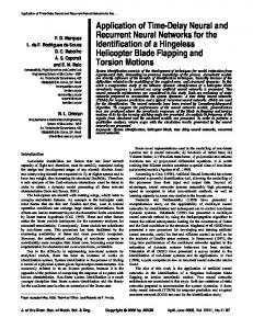
(b) Learning time ceeded in 41 trials out of 50 trials (Fig. 9a), and failed in 9 trials (Fig. 9b). Initially, the FAN has uniformly randomly distributed rate values between -1 and 1. After successful training, the dynamic activation rate r evolved to highly positive values (Fig. 9a, 1640 neurons from 41 trials). The number of neurons that have high r (i.e. between 0.5 and 1.0) increased, while neurons with negative r were reduced. This means that extrapolation is pushed to the max (Eq. 2), suggesting that neuroevolution tried to utilize the extrapolating dynamics as much as possible. In failed trials (Fig. 9b, 360 neurons from 9 trials), the neurons failed in evolving facilitating dynamics. The networks seemed to try to push down the decaying dynamics. (Notice the decreased number of neurons which have low r value (below -0.5) in the final state). However, most neurons maintained negative values of r. This suggests that decaying activity did not help to overcome neural delay. In sum, experiments with various forms of delay have shown that networks with facilitatory neurons were most effective in compensating for neural transmission delay. Also, the convergence of dynamic activation rate to high values shows that extrapolation is heavily utilized in FAN. Thus, facilitatory neural dynamics can be an effective way of keeping an organism’s internal state aligned with the environment, in the present. Finally, these dynamics can also contribute in dealing with external delay and uncertainty as shown in Fig. 8.
Figure 8: Blank-out test. tion weights and dynamic activation rates of the neurons were stored. Then, the successful FAN and control networks were loaded and tested under blank-out condition, respectively. (Note that 50 successful networks from FAN and control were tested.) As shown in Fig. 8(a), FAN showed higher performance than control network and slow decrease in performance until 600 ms (60 steps), which is surprisingly similar to the observation in human experiments. Also, the learning time is significantly faster than control networks as shown in Fig. 8(b). Note that the control network showed a steep decrease in performance and could not solve the problem beyond 70 steps (i.e. 700 ms) blank-out duration (success rate = 0 in Fig. 8(a)). Experiments with blank-out test have shown that FAN can also effectively deal with external delay by utilizing its extrapolatory neural activity.
4.4
Contribution of Dynamic Activation Rate
The performance results reported in the previous sections suggest that the dynamic activation rate r coded in the gene of the FAN controller serves a useful purpose. To verify if indeed the rate parameters are being utilized and, if it is, which neural dynamic (facilitating or decaying) is being developed, we looked at the evolution of these parameters over the generations. Fig. 9 shows the evolution of the rate parameters in FAN from successful networks. The distribution of initial and evolved dynamic activation rates are shown for a sample subpopulation. Each subpopulation, from which one neuron was drawn to participate in a network, consisted of 40 neurons. In this experiment, θz was delivered with delay, beginning from 50 steps and lasting until 150 steps within each generation. FAN suc-
5.
DISCUSSION
The main contribution of this paper was to propose a biologically plausible neural mechanism at a single neuron level for compensating for neural transmission delay. We developed a continuous-valued neuron model utilizing facilitatory dynamics which was able to perform robustly under internal sensory delay in the 2D pole-balancing task.
172
Because facilitation occurs at the cellular level, delay compensation is achieved faster than when it is done at a network level. Our experiments showed that a recurrent neural network with facilitatory single neuron dynamics took less time to learn to solve the pole-balancing problem with input delay and showed higher performance than the networks having only recurrent network dynamics. In the future, it would be interesting to test the effects of the number of hidden neurons and network topology on FAN’s performance. Another possibility is to use a feedforward network. However, it was shown that, for control networks, fully recurrent topology outperforms feedforward structure under limited input condition (i.e. only four inputs without velocity information) [15]. In this paper, we used continuous-valued neurons where the neural activity was represented as a single real number. However, biological neurons communicate via spikes, so the biological plausibility of the simulation results above may come under question. One potential instrument is the synaptic dynamics of facilitating synapses found in biological neurons (as we briefly mentioned in Sec. 2). These synapses generate short-term plasticity which shows activitydependent decrease (depression) or increase (facilitation) in synaptic transmission occurring within several hundred milliseconds from the onset of activity (for reviews see [19, 9]). Especially, facilitating synapses cause augmentation of postsynaptic response through increasing synaptic efficacy with successive presynaptic spikes. Such mechanism may be the neural basis of FAN. Preliminary results for this idea can be found in [20]. Also, such a neural mechanism implemented at the single-neuron level can be extended to multiple neurons. For example, in [21], we showed that facilitating synapses, together with adaptation through SpikeTiming-Dependent Plasticity (presynaptic), can serve as a neural basis for delay compensation in a network of bilaterally connected orientation-tuned cells. It would be worthwhile to verify further whether the dynamic activation rate r defined in Eq. 5 is plausible in terms of neurophysiology. It is known that facilitation is driven by elevated calcium levels in presynaptic terminals. Recently, a neurophysiological mechanism (e.g., involving calcium chelator BAPTA) has been found, which may be responsible for the regulation of the increase rate of synaptic efficacy [27]. Another question at this point relates to the extrapolatory capacity of facilitating neural dynamics. Extrapolation is usually related to prediction of the future from information from the present. However, in the nervous system, due to the neural transmission delay, extrapolation was used to predict the present based on past information. The question is, is it possible that neural mechanisms that initially came about for delay compensation could have developed further to predict future events? Prediction or anticipation of future events is an important characteristic needed in mobile, autonomous agents [24, 17]. One prominent hypothesis regarding prediction is the internal forward model [35]: Forward models existing in various levels in the nervous system are supposed to produce predictive behaviors which are based on sensory error correction. Internal forward models were suggested from an engineering point of view, where the sensory motor system is regarded as a well-structured control system that can generate accurate dynamic behaviors. Even though theoretical mechanisms similar to Kalman filter methods were
suggested [23], the precise neural basis for the forward models have not been fully investigated. Recently, several brain imaging studies provided supporting evidence for the existence of internal forward models in the nervous system [2, 33]. However, these results did not suggest what could be the neural substrate. Thus, it may be worthwhile investigating how such abilities in autonomous agents can be related to facilitatory dynamics at the cellular level. The input blankout experiment conducted in Sec. 4.3 is a first step in this direction, where delay compensation mechanisms evolved to deal with internal delay can be directed outward to handle environmental uncertainty. There are other forms of delay compensation such as increased myelination of axons, increase in the thickness of axons and dendrites, and changing the type of ion channels [8, 28]. However, there is a clear limit in the amount of compensation these processes can bring about, thus facilitating neural dynamics may still be needed. As we mentioned earlier, the dynamic activation rate may be an adaptable property of neurons, thus the rate may be adjusted to accommodate different delay durations. That way, organisms can cope with delay during growth. In our research, we focused on the dynamics of single neurons only. In principle, extrapolation can be done at a different level such as the local circuit level or large-scale network level. However, our view is that to compensate for delays existing in various levels in the central nervous system and to achieve faster extrapolation, the compensation mechanism needs to be implemented at the single-neuron level.
6.
CONCLUSION
In this paper, we have shown that facilitatory (extrapolatory) dynamics found in facilitating synapses may be used to compensate for delay at a single-neuron level. Experiments with a recurrent neural network controller in a modified 2D pole-balancing problem with sensory delay showed that facilitatory activation greatly helps in coping with delay. The same mechanism was also able to deal with uncertainty in the external environment, as shown in the input blank-out experiment. In summary, it was shown that facilitatory neural activation can effectively deal with delays inside, and outside, the system, and it can very well be implemented at a single neuron level, thus allowing a developing nervous system to be in touch with the present.
7.
ACKNOWLEDGMENTS
We would like to thank Faustino Gomez and Risto Miikkulainen for allowing us to use their ESP code.
8.
REFERENCES
[1] C. W. Anderson. Learning to control an inverted pendulum using neural networks. IEEE Control Systems Magazine, 9:31–37, 1989. [2] S.-J. Blakemore, D. M. Wolpert, and C. D. Frith. Central cancellation of self-produced tickle sensation. Nature neuroscience, 1:635–640, 1998. [3] Y. Choe. The role of temporal parameters in a thalamocortical model of analogy. IEEE Transactions on Neural Networks, 15:1071–1082, 2004. [4] D. Eagleman and T. J. Sejnowski. Motion integration and postdiction in visual awareness. Science, 287:2036–2038, 2000.
173
[5] J. L. Elman. Finding structure in time. Cognitive Science, 14:179–211, 1990. [6] J. L. Elman. Distributed representations, simple recurrent networks, and grammatical structure. Machine Learning, 7:195–225, 1991. [7] W. Erlhagen. The role of action plans and other cognitive factors in motion extrapolation: A modelling study. Visual Cognition, 11:315–340, 2004. [8] C. W. Eurich, K. Pawelzik, U. Ernst, J. D. Cowan, and J. G. Milton. Dynamics of self-organized delay adaptation. Physical Review Letters, 82:1594–1597, 1999. [9] E. S. Fortune and G. J. Rose. Short-term synaptic plasticity as a temporal filter. Trends in Neurosciences, 24:381–385, 2001. [10] Y.-X. Fu, Y. Shen, and Y. Dan. Motion-induced perceptual extrapolation of blurred visual targets. The Journal of Neuroscience, 21, 2001. [11] G. Fuhrmann, I. Segev, H. Markram, and M. Tsodyks. Coding of temporal information by activity-dependent synapses. Journal of Neurophysiology, 87:140–148, 2002. [12] W. Gerstner. Hebbian learning of pulse timing in the barn owl auditory system. In W. Maass and C. M. Bishop, editors, Pulsed Neural Networks, chapter 14, pages 353–377. MIT Press, 1998. [13] F. Gomez. Robust Non-Linear Control Through Neuroevolution. PhD thesis, Department of Computer Science, The University of Texas at Austin, Austin, TX, 2003. Technical Report AI03-303. [14] F. Gomez and R. Miikkulainen. 2-D pole balancing with recurrent evolutionary networks. In Proceeding of the International Conference on Artificial Neural Networks (ICANN), pages 758–763. Elsevier, 1998. [15] F. Gomez and R. Miikkulainen. Solving non-markovian control tasks with neuroevolution. In Proceedings of the International Joint Conference on Artificial Intelligence (IJCAI), Denver, CO, 1999. Morgan Kaufmann. [16] F. Gomez and R. Miikkulainen. Active guidance for a finless rocket through neuroevolution. In Proceedings of the Genetic and Evolutionary Computation Conference (GECCO), pages 2084–2095, Chicago, IL, 2003. Springer. [17] H.-M. Gross, A. Heinze, T. Seiler, and V. Stephan. Generative character of perception: A neural architecture for sensorimotor anticipation. Neural Networks, 12:1101–1129, 1999. [18] D. Kerzel and K. R. Gegenfurtner. Neuronal processing delays are compensated in the sensorimotor branch of the visual system. Current Biology, 13:1975–1978, 2003. [19] J. Liaw and T. W. Berger. Dynamic synapse: Harnessing the computing power of synaptic dynamics. Neurocomputing, 26-27:199–206, 1999. [20] H. Lim and Y. Choe. Facilitatory neural activity compensating for neural delays as a potential cause of the flash-lag effect. In Proceedings of the International Joint Conference on Neural Networks (IJCNN), pages 268–273. IEEE, 2005. [21] H. Lim and Y. Choe. Delay compensation through
[22]
[23]
[24]
[25] [26]
[27]
[28]
[29]
[30]
[31] [32]
[33]
[34]
[35] [36]
174
facilitating synapses and stdp: A neural basis for orientation flash-lag effect. In Proceedings of the International Joint Conference on Neural Networks (IJCNN). IEEE, 2006, In press. H. Markram, Y. Wang, and M. Tsodyks. Differential signaling via the same axon of neocortical pyramidal neurons. In Proceedings of the National Academy of Sciences, USA, volume 95, 1998. B. Mehta and S. Schaal. Forward models in visuomotor control. Journal of Neurophysiology, 88:942–953, 2002. R. M¨ oller. Perception through anticipation: An approach to behavior-based perception. In Proceedings of New Trends in Cognitive Science, pages 184–190, 1997. R. Nijhawan. Motion extrapolation in catching. Nature, 370:256–257, 1994. W. H. Press, B. P. Flannery, S. A. Teukolsky, and W. T. Vetterling. Numerical Recipes in FORTRAN: The Art of Scientific Computing. Cambridge University Press, Cambridge, UK, 2nd edition, 1992. A. Rozov, N. Burnashev, B. Sakmann, and E. Neher. Transmitter release modulation by intracellular ca2+ buffers in facilitating and depressing nerve terminals of pyramidal cells in layer 2/3 of the rat neocortex indicates a target cell-specific difference in presynaptic calcium dynamics. Journal of Physiology, 531:807–826, 2001. M. Salami, C. Itami, T. Tsumoto, and F. Kimura. Change of conduction velocity by regional myelination yields constant latency irrespective of distance between thalamus and cortex. In Proceedings of the National Academy of Sciences, USA, volume 100, pages 6174–6179, 2003. G. Silberberg, C. Wu, and H. Markram. Synaptic dynamics control the timing of neuronal excitation in the activated neocortical microcircuit. The Journal of Physiology, 556:19–27, 2004. K. O. Stanley and R. Miikkulainen. Efficient reinforcement learning through evolving neural network topologies. In Proceedings Genetic and Evolutionary Computation Conference (GECCO), pages 1757–1762, San Francisco, CA, 2002. Morgan Kaufmann. S. J. Thorpe and M. Fabre-Thorpe. Seeking categories in the brain. Science, 291:260–263, 2001. D. Wang. Temporal pattern processing. In M. A. Arbib, editor, The Handbook of Brain Theory and Neural Networks (2nd edition), pages 1163–1166. MIT Press, Cambridge, MA, 2003. B. Webb. Neural mechanisms for prediction: do insects have forward models? Trends in Neurosciences, 27:278–282, 2004. D. Whitney and I. Murakami. Latency difference, not spatial extrapolation. Nature Neuroscience, 1:656–657, 1998. D. M. Wolpert and J. R. Flanagan. Motor prediction. Current Biology, 11(18):R729–R732, 2001. X. Yao. Evolving artificial neural networks. Proceedings of the IEEE, 87:1423–1447, 1999.