Research Institute of Applied Economics 2009
Working Papers 2009/05, 27 pages
Factors explaining urban transport systems in large European cities: A cross-sectional approach
By Daniel Albalate1 and Germà Bel2 1
GiM - IREA. Departament de Política Econòmica, Universitat de Barcelona. Avda. Diagonal, 690. 08034 Barcelona, Spain. Email:
[email protected]. Telf: +34.93.4021945. 2
GiM - IREA. Departament de Política Econòmica, Universitat de Barcelona. Avda. Diagonal, 690. 08034 Barcelona, Spain. Email:
[email protected]. Telf. +34.93.4021946; Fax: 34.934024573
Abstract: The paper analyses the link between human capital and regional economic growth in the European Union. Using different indicat The importance of effective and efficient mobility in large cities is becoming essential for planners and citizens due to its impact in terms of social, economic and geographic development. The aim of this research is to determine factors explaining urban transport systems by estimating aggregate supply and demand equations for 45 large European cities. Supply and Demand equations are separately and jointly determined using OLS and SUR estimation models. On one hand, our findings suggest the importance of economic variables on the supply of public transport. On the other, we highlight the role of those factors influencing the generalized cost of transport as main drivers of demand for public transit. Additionally, regional variables are introduced to capture institutional heterogeneity in this service, and we find that regional patterns are powerful explanatory determinants of urban transportation systems in Europe. . Key words: Urban transportation, Local government policy, Mobility. . JEL codes: L91; L98; R41.
1
1. Introduction. Mobility is becoming increasingly essential in large cities as a consequence of its impact on social, economic and geographic development. In fact, transportation potentially affects the nature of the urban area itself, (Small, 1997; p. 253) and for this reason the literature on the relationship between travel behavior and urban form has grown at a fast pace during recent decades (Rodríguez, Targa and Aytur, 2006).1 Indeed, citizens in developed economies understand mobility as a right, especially in large cities where congestion and pollution make private transportation more inconvenient and expensive. In such urban environments, transport effectiveness and efficiency not only affect local and regional productivity rates, they also have an impact on citizens’ quality of life. The aim of this paper is to identify those factors explaining urban transport systems of large European cities from both the supply and demand sides. In this effort, we characterize aggregate supply and demand equations, which are separately (OLS) and jointly estimated (SUR), and we test the impact of well-known determinants as well as new explanatory variables that suggest interesting relationships between urban transport development and regional heterogeneity. The contribution of the present paper relies on the fact that, to our knowledge, this is the first study attempting to explain urban transportation systems from both demand and supply sides by using a cross-European sample of large cities.2 Taking into account supply and demand together, and enjoying a European-wide database of large cities, produces results of interest to both scholars and policy makers. Moreover, this analysis provides some new insights into the current literature on urban transportation. Notably, regional
1 Some relevant works are Sasaki (1990), Banister (1995), Banister, Watson and Wood (1997), Giuliano and Narayan (2003). 2 Gordon and Willson (1984) also used an international data set (data for 1978) of metropolitan cities but they only focused on light rail transport and estimated a semilog model of its demand (ridership per Km of lane) with only four exogenous variables. Moreover, they did not carry any analysis on supply determinants.
2
regularities in the basics of transport systems seem to emerge and reflect institutional heterogeneity in Europe. The rest of the current study is organized as follows. The next section is a brief review of the literature on urban transportation. Section 3 describes the empirical strategy pursued to determine transport supply and demand equations. Here we offer detailed information on the data and variables used, and the methodology applied. The fourth section presents the main results, and the last section (Section 5) concludes with some final remarks on our findings. 2. Related literature. The literature on public transport demand and supply enjoys a long tradition in the field of transport economics. Nonetheless, given the local dimension of the service, most studies have considered only single metropolitan areas, regions or countries for their analysis. As a consequence, few studies use international samples, and within this group, most studies are constructed as meta-analyses derived from different national or local studies. Price and time elasticities, modal choice and externalities internalization have been the leading topics in the recent literature on urban public transport demand. The work by Dargay and Hanly (2002) uses data on English counties to estimate a dynamic relationship between per capita bus patronage and bus fares. Their work distinguishes between the short and long-term impact of fare changes on bus patronage--as do most studies on this issue--and provides an indication of the time required for the total response to occur. Matas (2004) also estimates an aggregate demand function for bus and underground trips in the metropolitan area of Madrid, Spain in order to obtain the demand elasticities of the main attributes of public transport services. The study’s second objective is to evaluate the impact on revenue of the introduction of the travel card scheme by estimating a matrix of own and cross-price elasticities for different ticket types. For the same metropolitan area
3
we have the recent study by García-Ferrer et al. (2006), which studies the incidence of alternative types of public transport modes. Hencher (1998) also distinguishes between fare classes across train and bus modes of public transportation and the car for commuting travel in the Sydney, Australia metropolitan area, while Marchese (2006) uses her theoretical model to show that integrated tariffs can be used to extract the consumer's surplus if there are a lot of connections supplied. The meta-analyses by Nijkamp and Pepping (1998), Kremers et al. (2002) and by Holmgren (2007) review the wide variation in demand elasticities found in the literature. The first focuses on price elasticity, while the latter also considers other elements. In fact, it sheds light on the importance of including car ownership, own price, income and some measures of service in demand models. Moreover, it supports the position that explanatory variables should be in per capita terms if population is not included in the model. Close to these studies but more focused on the determinants of demand of public transport, we find Paulley et al. (2006), which concentrates on the influence of fares in the UK, though it also studies the roles played by quality of service, income and car ownership. Related to this last element, Bresson et al. (2004) present a panel data analysis for French urban areas, finding a clear downward trend in public transport patronage that is mainly due to increasing car ownership. In addition, the use of public transport appears to be quite sensitive to the volume supplied and its price, which makes the financial equilibrium of this industry problematic. Regarding mode choice we can mention the recent study by Sungyop and Ulfarsson (2008), which analyzes transportation mode choice for short home-based trips using a survey from a part of Washington State, or the paper by Asensio (2002), which reveals elasticities for commuters using different modes in Barcelona, Spain.
4
Finally, a large group of recent theoretical and empirical studies have worked on pricing schemes to internalize the external costs of transport by linking subsidies, price of public transport and road charges. De Borger et al. (1996) develop a simple theoretical model that determines optimal prices for private and public urban transport services, taking into account all relevant private and external costs. Similar works with relevant extensions can be found in De Borger, Kerstens and Costa (2002), Pedersen (2003), Small (2004), and Parry and Small (2007), among others. On the supply side we find that technical efficiency and determinants of production cost structure have been the main foci of study. Less common are works on the determinants of transport supply systems. To this extent, Brueckner and Selod (2006) recently advanced the construction of a political economy model where transport system (supply) is endogenously determined. Nonetheless, no empirical strategy is used to test their hypothesis. De Borger and Wouters (1998) also simulate a model on supply decisions based on the influence of prices and traffic flows in Belgium, but further research on these determinants is needed. Others like Fernández, Cea and de Grange (2005) and Fernández, de Cea and Malbran (2008) have also recently made efforts to link demand responsiveness to supply design. On the other hand, we find many relevant works on cost structure and technical efficiency. The work of Farsi, Fetz and Filippini (2007), analyzes the cost structure of the Swiss urban public transport sector in order to assess scale and scope economies. The significant economies of scope estimated favor integrated multi-mode operations as opposed to unbundling. On the other side, Van Reeven (2008) shows that economies of scale do not constitute a justification for general subsidization of urban public transport. The same result was already found in Matas and Raymond (1998) for the Spanish case. Furthermore, Roy and Yvrande-Billon (2006) use data on French municipalities to estimate a stochastic frontier model that corroborates that technical efficiency of urban
5
public transport operators depends on their ownership regime and the type of contract governing their transactions. This brief presentation of the main groupings of work in the field of urban transportation systems highlights the relevance of the analysis we propose. This study is embedded within the literature on the determinants of urban public transport demand and supply. Its main contribution relies on being the first study that uses a rich international sample of large European cities (with detailed information on the local basis for the whole transportation system: bus, light rail, metro, tram, etc.) in order to estimate separately and simultaneously both aggregate demand and supply equations. This is especially relevant since past literature has been analyzed these equations separately, focused on one or two modes of public transport, and treated single region samples. Additionally, we make an effort to capture and compare different institutional or regional frameworks that, as we will make clear, seem to play an important role in the determination of transport systems across the continent. This opening up of regional heterogeneity in urban transportation is possible thanks to the international nature of our sample, and provides promising results that can stimulate future research. 3. Empirical Strategy. In this section we describe the data and the model we have used to explain the demand and supply sides of urban transport systems in European cities. 3.1 Data The data used in this research is obtained from the Mobility in Cities Database (MCD) provided by the International Association of Public Transport (UITP). This database offers 120 indicators of public transport (not, unfortunately, including ownership data) from 50 worldwide cities in 2001, most in Europe. In order to improve the homogeneity of the sample, we use only the data from 45 European cities.
6
Table 1 reports the cities and some of their socio-demographic characteristics in order to illustrate the variability of our sample. Table 2 classifies these cities by region to show that our sample uses cities of sufficient variety to capture a wide range of social and economic attributes and heterogeneous institutional frameworks and avoid results led by certain types of cities. In spite of this, we must acknowledge that the weights of Mediterranean and Center-European metropolitan areas are slightly higher than the rest of regional groups (Nordic, Atlantic and Eastern). > 3.2 The Model In this study we attempt to estimate both aggregate supply and demand equations for urban transport for our 45 European cities. On one hand, our supply equation can be considered as a production function of urban transport expressed in the following form: Supply = f ( income, operational_costs, phisical_capital, city_characteristics)
(1)
Therefore, supply for urban transport is supposed to rely on the recovery rate of the service by the producer (income over costs), by the fleet of vehicles (capital), and other city characteristics like economic activity or density.3 On the other hand, the aggregate demand for transport services can be assumed to depend on the attributes of the service affecting the generalized cost of transport (monetary cost, time cost,.…), but also on the properties of the alternative modes and city characteristics as well. For this reason our demand equation considers all these factors by assuming they can be expressed as an extension of the generalized transport cost equation, which can be assumed to follow the next form: Demand = h ( price, time, city_characteristics)
(2)
The labor factor can be considered to be included in the operational costs variable. City characteristics could have a significant impact on supply given the needs of citizens, or due to their impact on efficiency and equity. 3
7
In this case demand is affected by the price of the service for the user, the time spent in the journey (walking time, waiting time, and in-vehicle time, and also taking into account the journey time in the alternative mode) and city characteristics. For this reason we will consider not only urban public transport variables, but also variables describing private transport and city characteristics that can capture these time dimensions. As a result, the equation system to be estimated in order to explain urban transport supply and demand for these 45 European cities can be expressed in the following double log form:
Supplyi = ln(
place − km )i = α + β1 ln(GDPi ) + β2 ln(DENSi ) + β3 ln(PRICEi ) + β4 ln(OCOSTi ) + population
β5 ln(FLEET )i + β6 Dcapitali + ε1
Demandi = ln(
(3)
passenger − km ) = δ + λ1 ln(GDPi ) + λ2 ln(DENSi ) + λ3 ln(PRICEi ) + λ4 (FLEETi ) + Population
λ5 ln(PUBSPEEDi ) + λ6 ln(PRIVATE _ TIMEi ) + λ7 ln(MOTORi ) + λ8 ln(PARKINGi ) + λ9 Dcapitali + ε2 (4)
where the first equation (3) refers to the supply equation and the second (4) to the demand equation. The sub-index i makes reference to each city. The double log specification facilitates the interpretation of the estimated coefficients in terms of elasticities and has been selected from among other functional forms due to its higher goodness of fit. The dependent variables are, respectively, the number of place-km per capita in the case of the supply equation, and the number of passenger-km per capita for the demand equation. Several variables enter as covariates in supply and demand equations in order to explain urban transport systems. The variables and their expected relationships with the dependent variables are described below.
8
GDP: Gross domestic product per capita. This variable captures income and economic activity. Richer cities can provide better and more extensive transport systems. At the same time mobility is positively correlated with the economic activity and for this reason we expect to confirm positive impacts on both demand and supply equations due to the introduction of this variable.4 DENS: Urban population density. This variable captures city characteristics and urban form. It is well known and widely recognized that mobility and mode choice is affected by city form (Nijkamp and Rienstra, 1996). Cameron, Kenworthy and Lyons (2003) stress that private motorized mobility, for instance, although arising from local decisions, is determined by the structure of the urban environment. In general, dense cities are associated with a high use of public transport (Newman and Kenworthy, 1989). Therefore, the choice between public and private transport systems is influenced by urban form. For this reason dense cities are expected to have large transport systems since supply becomes profitable (or less expensive) by taking advantage of scale and density economies. In addition, density is expected to explain both transport demand and supply. In the case of demand it is worth pointing out that the expected positive correlation that exists between dense cities and short distances to public transport stations implies a negative correlation between dense cities and walking time, which is one of the temporal dimensions of the generalized cost of travel. PRICE: Average price charged to urban transport users. Prices are usually regulated by public authorities and are rarely driven by market (demand) forces. This is usually considered a political price and for this reason we do not suffer from endogeneity problems in the supply equation by its presence. This rigidity makes us expect no influence of prices on transport supply because public transport in Europe is highly subsidized and regulated. Concretely, the average subsidy in Europe is 48% according to UITP (2005) It is important to highlight that the database “Mobility in Cities” does not contain information related to personal income in these cities, which is a variable usually introduced in this kind of transport models. 4
9
estimates. On the other hand, prices always affect individual demand decisions, and for this reason we will expect strong impacts on transport aggregate demand. OCOST: Average operating cost of one public transport place-km. This variable reflects the operating cost of providing each place-km. For this reason we expect a negative relationship between the operational cost and transport supply. The more expensive the place –km is, the lower the number of place-kms offered by public authorities. FLEET: The fleet of vehicles available for public transport purposes. Within this category we include the number of buses, metro wagons, and trams. The higher the number of vehicles, the higher the expected number of place-km per capita offered in the system. Also, more vehicles imply better service since number of vehicles is associated with frequency, which captures another temporal dimension (waiting time) and can be also decrease congestion, resulting in the service being more comfortable. Given this rationale, we expect higher transport demand. Therefore, this variable is expected to affect both equations positively. Dcapital: A dummy variable taking value one if the city is a political capital and zero otherwise. By using this variable we are interested in possible biases derived from politics and from administrative services, as well as from other specific characteristics of political capitals. PUBSPEED: Average speed of public transport vehicles in operation. Speed is associated with service quality and is correlated to “in vehicle” time. Since this is extremely related to time savings, it becomes an essential factor of the generalized costs of transport equation. A consequence, we expect positive relationships between speed and transport demand.5 PRIVATE_TIME: Average time spent by private vehicle trip. Time spent in private transport has an increasing impact on demand for public transport since private transport is negatively related to public transport demand as a substitute commodity. Therefore, it is One can argue that speed also affects transport supply since it decreases operational costs. However, we already introduce the operational cost in the supply equation. 5
10
a relevant factor of the generalized transport cost equation for the traveler since it captures the opportunity cost--in terms of time--of choosing public transport. As private journey duration grows, then public transport, at a reasonable speed, becomes relatively more convenient for the traveler. MOTOR: Motorization constructed as the number of private vehicles per thousand populations. More private vehicles tend to lower incentives to use public transport. For this reason we expect negative relationships between car ownership and public transport demand.6 However, there is an important caveat. This figure reflects the motorization of the metropolitan area, but private transport from outside the limits of the metropolitan area is to be expected. For this reason our variable cannot capture the whole participation of private vehicles in the metropolitan area, but it does represent an important share. PARKING: The number of parking spaces per thousand jobs in the Central Business District. This indicator offers information on private transport convenience for the traveler needing mobility to work. Parking space is an essential factor in private transport choice. As a result, we expect negative impacts on demand for public transport as parking spaces increase. Button (2006) recognizes the importance of this necessary supply, since he suggests that automobiles spend over 95% of their time ‘parked’, and trucks over 85%. Descriptive statistics and expected signs associated with the variables defined above, are displayed in table 3. > 4. Estimation and Results. We first estimate our equation system using the Heteroskedasticity-Robust Ordinary Least Squares estimator (OLS) for each equation separately. Afterwards we implement a SUR model (Seemingly Unrelated Regression, also called joint generalized least squares or Low supply of public transport could increase the need of having private vehicles to travel. In this sense, motorization would be affected by public transport supply. The inverse relationship is not so clear. For this reason we avoid the use of motorization in the supply equation. In fact, even when we introduce this variable our results do not change and motorization itself is not statistically significant at all.
6
11
Zellner estimation), which jointly estimates the equation system allowing for correlation between error terms through equations.7 This last strategy is used when is unrealistic to expect that in a set of equations, errors would be uncorrelated. This is in turn a more efficient estimator than OLS. Indeed, substantial efficiency gains are expected while contemporaneous disturbances in different equations are highly correlated.8 The SUR method uses the correlations among the errors in different equations to improve the regression estimates, but requires an initial OLS regression to compute residuals. The OLS residuals are used to estimate the cross-equation covariance matrix. Indeed, it is very likely that some factors not included in the equation may affect both urban supply and demand. Table 4 displays our results for separate and joint estimations. Overall explanatory power is high for every method of estimation and for every equation, especially for those of demand. As results show, the goodness of fit of the models is satisfactory for each separate equation and for the joint estimation as well. Moreover, no substantial differences are found between OLS and SUR estimates, which imply that OLS was already highly efficient in our case. Interesting results arise from our estimations. In separate estimations we find that GDP, the number of total vehicles supplied and being a political capital all produce positive impacts on the supply side of transport systems across the 45 European cities. On the other hand, the operational cost of the service is the main variable pushing to negatively affect place-km per capita. The other variables, including the average price of a passengerkm and urban population density, do not present statistically significant coefficients. This result of fare effects on supply is not strange if we consider that prices are highly regulated and usually driven political goals, not operational costs. At the same time, urban population density was thought to affect supply through its impacts on economic efficiency, but its
7 8
In SUR strategy the equations are estimated as a set in order to increase efficiency. See the seminal work by Zellner (1962) on Seemingly Unrelated Regression Equations.
12
coefficient does not seem statistically significant at all. It is possible that urban population density is not able to capture urban form by itself. Regarding demand equations we find that coefficients associated with GDP, with the fleet of vehicles provided, being a political capital, and the average time spent in private transport trips, are all positively correlated with passenger-km per capita. On the other hand, the average price of public transport and the number of parking spaces in the central business district have statistically significant but negative impacts on public transport demand. All impacts work in the expected direction. The rest of variables do not provide any statistically significant coefficients. In fact, motorization in the metropolitan area does not seem to explain public transport demand. Probably, this lack of statistical impact--though we find the expected sign--is be driven by the traffic coming from outside the metropolitan area boundaries. While public transport is used more often to undertake short daily trips, private transport tends to be more present in long daily journeys. For this reason, and given the absence of statistical significance, we replicate the same joint estimation--specifications 5 and 6--without the variable MOTOR.9 As is shown, the explanatory power of this estimation remains the same and several coefficients improve their statistical significance. Particularly, we find that the average speed of public transport is now statistically significant at 10%. Furthermore, paying attention to the differences between the SUR and OLS estimations, we realize that the results displayed provide few and almost insignificant changes on the statistical significance of the coefficients related to the variables used in the separate models. For this reason we know that there are efficiency gains from the use of SUR models, but these are rather small.
It is worth saying that even motorization is removed, we still keep two variables related to private transport. These are the duration of private trips and the number of parking spaces in the central business district. 9
13
Once we have determined the main factors affecting urban transportation supply and demand from a statistical point of view, we attempt to replicate the estimation by introducing regional dummies. By doing this we wish to identify any regional effect or regularity having an impact on urban transportation systems. The dummy variables chosen recognize the distribution made in table 2 and their description is the following: DSOUTH: A binary variable identifying cities close to the Mediterranean Sea with value 1, and 0 otherwise. This variable includes cities from France, Greece, Italy, Portuga,l and Spain. DCENTER-EUROPEe: A binary variable identifying cities from the center of the European continent with value 1 and 0 otherwise. In this category we find cities from Austria, Belgium, France, Germany, Switzerland, and the Netherlands. DNORTH: A binary variable identifying cities from the north of the continent (Nordic and Atlantic cities) with value 1 and 0 otherwise. In this category we find cities from Denmark, Finland, Ireland, Norway, Sweden, and the United Kingdom. DEAST: A binary variable identifying cities from the east of the continent (former Popular Republics) with value 1, and 0 otherwise. The variable includes cities from Czech Republic, Estonia, Hungary, Poland, and Russia. Since we enjoy few degrees of freedom, we introduce these regional dummies step by step in order to compare the region chosen with the rest of regional groups. We present the results derived from this strategy in table 5. Thus, this extends equations 3 and 4 with another dummy variable. First of all, it is important to mention that all the other covariates are introduced in the specification and we don’t find any significant change in the statistical impacts of their coefficients on our dependent variables. This being said, we can analyze the selected results of table 5, and see that Mediterranean metropolitan areas have lower levels of public transport supply and demand than do the rest of regions as a whole. In contrast, Center-
14
European cities enjoy higher public transport supply and demand. The coefficient associated with the Northern cities does not appear to be statistically significant in the supply and demand equations, while Eastern cities provide mixed results. On one hand, these cities seem to deliver higher supply than the other groups. On the other, the coefficient is not statistically significant in the demand equation. We must take into consideration that the number of observations in this last couple of regions is smaller and we should be cautious about extracting general conclusions. Nevertheless, institutional and cultural characteristics seem to play a role in the determination of the urban public transport system in the cities considered. These results suggest the direction chosen by each region. To go deeper into regional effects, we provide Non-parametric analysis (kernel densities) that relates the supply of urban public transport in the cities of our sample with their geographical latitude and longitude. Figures 1 and 2 show the results of those kernel densities. > As the reader can observe, we find an inverted U-shape relationship between urban public transport supply and both geographical longitude and latitude. This means that the higher supply is expected in cities in the center of the continent. Therefore, we find a center-periphery scenario that tends to have its center on cities between 0º-10º of longitude and between 45º and 55º of latitude. The cities within this area are: Paris, ClermontFerrand, Ghent, Lille, Amsterdam, Brussels, Lyon, Rotterdam, Geneva, Bern, Turin, Zurich, Hamburg, Milan, and Stuttgart. Departing from this area, both Northern and Southern cities and both Western and Eastern cities seem to provide lower supply per capita. Regarding geographical longitude, we realized that western cities (Irish, British, Portuguese and most Spanish) provide low urban public transport supply per capita. However, the level served is higher than the one delivered by Eastern cities.
15
5. Conclusions With our analysis we identify the determinants of urban transport systems. We contribute to the existing literature by explaining urban transport systems from both demand and supply sides, and by using a cross-European sample of large cities. Interesting results arise from our estimations on factors explaining urban transport systems. The supply side of transport system is positively affected by Gross Domestic Product, the number of total vehicles supplied, and being a political capital. On the contrary, a negative effect on supply is exerted by the operational cost of the service. Regarding demand equations we find that coefficients associated with GDP, with the fleet of vehicles provided, being a political capital, and the average time spent in private transport trips, are all positively correlated with passenger-km per capita. On the contrary, the average price of public transport and the number of parking spaces in the central business district have negative effects on public transport demand. Besides analyzing the main determinants of urban transportation supply and demand, we identify regional effects having an impact on urban transportation systems. CenterEuropean cities enjoy higher levels of public transport supply and demand. On the contrary, Mediterranean metropolitan areas provide lower levels of public transport supply and demand than the remaining regions as a whole. Eastern cities provide mixed results, since they deliver higher supply than the remaining groups, but the coefficient in the demand equation is not statistically significant. Overall, we find an inverted U-shape relationship between urban public transport supply and both geographical longitude and latitude; the highest supply is expected in cities placed in the center of the continent. Our analysis provides interesting results and new insights that contribute to the current literature on urban transportation. Besides factors explaining supply and demand for transport systems, we have found regional patterns. Indeed, regional regularities appear to emerge and to reflect institutional heterogeneity in Europe.
16
Acknowledgements We are thankful for financial support from the Spanish Commission of Science and Technology (SEJ2006-04985). We are also grateful to comments and suggestions from Xavier Fageda.
References Asensio, J., 2002.Transport Mode Choice by Commuters to Barcelona's CBD. Urban Studies 39(10), 1881-1895. Banister, D., 1995. Transport and urban development. E&FN Spon, London. Banister, D., Watson, S., Wood, C, 1997.Sustainable cities: transport, energy and urban form. Environment and Planning B 24(1), 125-143. Bresson, G., Dargau. J., Madre, J., Pirote, A., 2004. Economic and structural determinants of the demand for public transport: an analysis on a panel of French urban areas using shrinkage estimators. Transportation Research Part A 38(4), 269-285. Brueckner, J, Selod, H., 2006.The political economy of urban transport-system choice. Journal of Public Economics 90(6-7), 983-1005. Button, K., 2006.The political economy of parking charges in “first” and “second-best” worlds. Transport Policy 13(6), 470-478. Cameron, I., Kenworthy, J, Lyons, T., 2008. Understanding and predicting private motorised urban mobility. Transportation Research Part D 8(4), 267-283. Dargay, J, Hanly, M., 2002.The demand for local bus services in England. Journal of Transport Economics and Policy 36(1), 73-91. De Borger, B., Kerstens, K., Costa, A., 2002. Public Transit Performance: What does One Learn from Frontier Studies? Transport Reviews 22(1), 1–38. De Borger, B., Mayeres, I., Proost, S, Wouters, S., 1996.Optimal pricing of urban passenger transport - A simulation exercise for Belgium” Journal of Transport Economics and Policy 30(1), 31-54 De Borger, B, Wouters, S., 1998. Transport externalities and optimal pricing and supply decisions in urban transportation: a simulation analysis for Belgium. Regional Science and Urban Economics 28(1), 163-197.
17
Farsi, M., Fetz, A, Filippini, M., 2007. Economies of scale and scope in local public transportation. Journal of Transport Economics and Policy 41(3), 345-361. Fernández, J., de Cea, J, de Grange, L., 2005. Production costs, congestion, scope and scale economies in urban bus transportation corridors. Transportation Research Part A 39(5), 383403. Fernández, J., de Cea, J, Malbran, R., 2008. Demand responsive urban public transport system design: Methodology and application. Transportation Research Part A 42(7), 951-972. García-Ferrer, A., Bujosa, M., de Juan, A, Poncela, P., 2006. Demand forecast and elasticities estimation of public transport. Journal of Transport Economics and Policy 40(1), 4567. Giuliano, G, Narayan, D., 2003. Another look at travel patterns and urban form: the US and Great Britain. Urban Studies 40(11), 2295-2312. Gordon, P, Willson, R., 1984. The determinants of light-rail transit demand––an international cross-sectional comparison. Transportation Research A 18(2), 135–140. Hensher, D., 1998. Establishing a Fare Elasticity Regime for Urban Passenger Transport. Journal of Transport Economics and Policy 32(2), 221–46. Holmgren, J., 2007. Meta-Analysis of Public Transport Demand. Transportation Research: Part A: Policy and Practice 41(10), 1021-35. Kremers, H. Nijkamp, P., Rietveld, P., 2002. A meta-analysis of price elasticities of transport demand in a general equilibrium framework. Economic Modelling 19(3), 463-485. Marchese C., 2006. The Economic Rational for Integrated Tariffs in Local Public Transport. Annals of Regional Science 40(4), 875-885. Matas, A., 2004. Demand and revenue implications of an integrated public transport policy: The case of Madrid. Transport Reviews 24(2), 195-217. Matas, A, Raymond, J., 1998. Technical characteristics and efficiency of urban bus companies: The case of Spain. Transportation 25(3), 243–263 Newman, P, Kenworthy, J., 1989. Gasoline consumption and cities; a comparison of US cities with a global survey. Journal of the American Planning Association 55(1), 24-37. Nijkamp, P, Pepping, G., 1998. Meta-analysis for explaining the variance in public transport demand elasticities in Europe. Journal of Transportation and Statistics 1(1), 1–14. Nijkamp, P, Rienstra, S., 1996.Sustainable transport in a compact city, in: Jenkins, M., Burton, E, Williams, K (eds.) The compact city; a sustainable urban form?, 190-199. Parry, I, Small, K., 2007. Should urban Transit Subsidies Be Reduced. University of California-Irvine, Department of Economics, Working Papers: 060723, 47 pages.
18
Paulley, N., Balcombe, R., Mackett, R., Titheridge, H., Preston, J., Wardman, M., Shires, J, White, P., 2006. The demand for public transport: The effects of fares, quality of service, income and car ownership. Transport Policy 13(4), 295-306. Pedersen, P., 2003. On the Optimal Fare Policies in Urban Transportation. Transportation Research B 37(5), 423–35. Rodríguez, D., Targa, F, Aytur, S., 2006. Transport implications of urban containment policies: A study of the largest twenty-five US Metropolitan Areas. Urban Studies 43(10), 1879-1897. Roy, W, Ybrande-Billon, A., 2007. Ownership, Contractual Practices and Technical Efficiency: The Case of Urban Public Transport in France. Journal of Transport Economics and Policy 41(2), 257-282. Sasaki, K., 1990. Income class, modal choice, and urban spatial structure. Journal of Urban Economics 27(3), 322-343 Small, K., 1997. Urban Transportation Economics. In: Arnott, R (ed.) Regional and Urban Economics: Encyclopedia of Economics, Part 1. Harwoord Economic Publishers, pp. 251-440. Small, K., 2004. Road pricing: Theory and evidence. In: Santos, G. (Ed.) Research in Transportation Economics 9. Oxford; Amsterdam and San Diego: Elsevier, JAI, pp. 133-158. Sungyop, K, Ulfarsson, G., 2008. Curbing Automobile Use for Sustainable Transportation: Analysis of Mode Choice on Short Home-Based Trips. Transportation 35(6), 723-737. UITP (2005) (International Association of Public Transport). Mobility in Cities Database, Mimeo. Van Reeven, P., 2008. Subsidisation of Urban Public Transport and the Mohring Effect. Journal of Transport Economics and Policy 42(2), 349-359. Zellner, A., 1962. An efficient method of estimating seemingly unrelated regressions and tests for aggregation bias. Journal of the American Statistical Association 57(298), 348-368.
19
TABLES Table 1. European cities in the database and socio-demographic characteristics Metropolitan Area
Population
GDP
Urban Pop. Density
Amsterdam
850 000
34 100
57.3
Athens
3 900 000
11 600
65.7
Barcelona
4 390 000
17 100
74.7
Berlin
3 390 000
20 300
54.7
Bern
293 000
35 500
41.9
Bilbao
1 120 000
20 500
51.9
Bologna
434 000
31 200
51.6
Brussels
964 000
23 900
73.6
Budapest
1 760 000
9 840
46.3
Clermont-Ferrand
264 000
24 200
44.5
Copenhagen
1 810 000
34 100
23.5
Dublin
1 120 000
35 600
25.9
Geneva
420 000
37 900
49.2
Gent
226 000
26 700
45.5
Glasgow
2 100 000
20 600
29.5
Graz
226 000
29 600
31
Hamburg
2 370 000
38 800
33.9
Helsinki
969 000
36 500
44
Krakow
759 000
7 010
58.4
Lille
1 100 000
21 800
55
Lisbon
2 680 000
17 100
27.9
London
7 170 000
36 400
54.9
Lyons
1 180 000
27 100
40
Madrid
5 420 000
20 000
55.7
Manchester
2 510 000
22 400
40.4
Marseilles
800 000
22 700
58.8
Milan
2 420 000
30 200
71.7
Moscow
11 400 000
6,060
161
Munich
1 250 000
45 800
52.2
Nantes
555 000
25 200
34.7
Newcastle
1 080 000
18 400
42.5
Oslo
981 000
42 900
26.1
Paris
11 100 000
37 200
40.5
Prague
1 160 000
15 100
44
Rome
2 810 000
26 600
62.6
Rotterdam
1 180 000
28 000
41.4
Sevilla
1 120 000
11 000
51.1
Stockholm
1 840 000
32 700
18.1
Stuttgart
2 380 000
32 300
35.3
Tallinn
399 000
6,880
41.9
Turin
1 470 000
26 700
46.1
Valencia
1 570 000
14 300
50.2
Vienna
1 550 000
34 300
66.9
Warsaw
1 690 000
13 200
51.5
Zürich 809 000 41 600 Source: Mobility in Cities Database (UITP)
44.5
20
Table 2. European cities in the database by region. Southern Athens Barcelona Bilbao Bologna Clermont-Ferrand Lille Lisbon Lyons Madrid Marseilles Milan Nantes Rome Seville Turin Valencia 16 (35%)
Center-Europe Amsterdam Berlin Bern Brussels Geneva Gent Graz Hamburg Lille Munich Paris Rotterdam Stuttgart Vienna Zürich
Northern Dublin Copenhagen Glasgow Helsinki London Manchester Newcastle Oslo Stockholm
Eastern Budapest Krakow Moscow Prague Tallin Warsaw
15 (33%)
9 (20%)
6 (13%)
21
Table 3. Independent variables. Definition, descriptive statistics and expected sign. Regressors
Definition
Mean
Std. Dev.
Max.
Min.
GDP DENS PRICE OCOST FLEET PUBSPEED PRIVATE_TIME PARKING MOTOR Dcapital
Gross Domestic Product per inhabitant (Euro) Urban population density Average cost of one public transport passenger-km for the traveler (0.01 Euro) Average operating cost of one public transport place-km (0.01 Euro) Total public transport vehicles per million inhabitants Average speed of public transport vehicles in operation (Km/h) Average duration of a private motorized trip (minutes) Number of parking spaces per thousand jobs in the Central Business District. Private passenger cars per thousand inhabitants Binary variable taking value 1 if the city is a political capital and 0 otherwise.
25 577 49.29 9.32 3.42 1,072 27.54 21.76 222.77 468 0.48
10 361 21.59 5.00 1.55 406 1.11 0.72 28.00 119 0.07
45 800 161.0 23 8.06 2,500 41.8 32 778 770 1
6,060 18.1 0.6 0.48 430 14.1 14 30 193 0
Impact Supply + + +/+
+/-
Impact Demand + + + + + +/-
22
Table 4. Least-squares estimates and Seemingly unrelated regression results (45 European cities) Separate Estimates (OLS)
Joint Estimates (SUR)
Joint Estimates (SUR)
Regressors
Supply (1)
Demand (2)
Supply (3)
Demand (4)
Supply (5)
Demand (6)
GDP
0.5671** ( 2.62) -0.1052 (-0.87) -0.4850*** ( -5.56) -
0.8230*** (4.88) 0.1399 (1.01) -0.0063 (-0.06) -0.6613*** (-4.85) 0.5021*** (3.94) 0.3488*** (3.16) -
0.5152*** (3.50) -0.0484 ( -0.36) -0.4939*** (-5.01) -
PRIVATE_TIME
-
MOTOR
-
PARKING
-
R2 Test F (Joint Significance) Chi2 (Joint Significance)
0.67 24.15***
0.3803** (2.67) 0.3166** ( 2.30) 0.4268 (1.11) 0.6097** ( 2.45) -0.3077 ( -1.30) -0.2076* ( -1.96) 0.86 46.65***
0.8378*** (4.95) 0.1442 (1.04) -0.0007 ( -0.01) -0.6837*** (-4.95) 0.5009*** (3.93) 0.3484*** ( 3.15) -
0.6222*** ( 3.46) -0.0498 (-0.37) -0.5264*** (-5.15) -
PUBSPEED
0.7469*** (4.27) 0.1798 ( 1.59) 0.0308 ( 0.28) -0.6840*** (-4.79) 0.5019*** (4.40) 0.3265** (2.57) -
-
-
DENS PRICE OCOST FLEET Dcapital
0.74 -
0.3774*** ( 2.79) 0.3902*** ( 3.43) 0.2225 ( 1.27) 0.3960* (1.85) -0.2206 (-1.31) -0.1549** (-2.49) 0.84 -
106.34***
219.75***
-
-
0.3637*** (2.68) 0.4135**** (3.62) 0.2860* (1.76) 0.3334* (1.69) -
0.74 -
-0.1726*** (-2.87) 0.84 -
105.42***
209.38***
Note 1. T-statistics and Z-statistics based on robust to heteroskedasticity standard errors are in parenthesis. Each model includes an intercept. Note 2. Significance at 1% (***), 5% (**) and 10% (*).
23
Table 5. Selected seemingly unrelated regression results by region (45 European cities). Regressor
DCENTER-EUROPE
Supply (5) -0.4364*** (-4.60) -
Demand (6) -0.3677*** (-2.82) -
DNORTH
-
DEAST R2 Chi2 (Joint Significance)
DSOUTH
Supply (7) -
Demand (8) -
Supply (9) -
Demand (10) -
Supply (11) -
Demand (12) -
0.2169** (2.32) -
-
-
-
-
-
0.2490*** (2.77) -
-
-
-
-
0.0213 (0.13) -
-
-
-0.0939 (-0.46) -
0.83 181.00***
0.85 235.27***
0.79 136.29***
0.86 233.66***
0.75 109.68***
0.84 207.25***
0.5248* (1.89) 0.76 119.00***
0.3712 (1.16) 0.84 211.32***
Note 1. Z-statistics based on robust to heteroskedasticity standard errors are in parenthesis. Each model includes an intercept and the rest of covariates. Note 2. Significance at 1% (***), 5% (**) and 10% (*).
24
Annex Table 6. Correlation matrix GDP DENS PRICE OCOST FLEET Dcapital PUBSPEED PRIVATE_TIME MOTOR PARKING
GDP 1 -0.4294 0.5280 0.6020 -0.0490 -0.0507 0.4072 -0.1483 0.3474 -0.1205
DENS
PRICE
OCOST
FLEET
Dcapital
PUBSPEED
PRIVATE_TIME
MOTOR
PARKING
1 -0.3668 -0.2286 -0.0407 0.1761 0.0816 0.3927 -0.2386 -0.0763
1 0.5357 -0.0668 -0.3809 0.0552 -0.4777 -0.0450 -0.1387
1 -0.1641 -0.2188 -0.1334 -0.1211 0.4301 0.0463
1 0.4586 0.0113 -0.1187 -0.1128 -0.3241
1 0.3083 0.2178 -0.2354 -0.2634
1 0.0792 -0.2467 -0.3743
1 0.1730 -0.2158
1 0.2812
1
25
FIGURES
0
.01
supply .02
.03
.04
Figure 1. Kernel density. Relationship between geographical longitude and public transport supply.
-10
0
10
20
30
40
longitude
Note: -
Cities between -9º and 0º (ordered by longitude degree): Lisbon, Dublin, Seville, Glasgow, Madrid, Bilbao, Manchester, Valencia, Newcastle, Nantes, London, Cities between 1º and 10º (ordered by longitude degree): Barcelona, Paris, ClermontFerrand, Ghent, Lille, Amsterdam, Brussels, Lyon, Rotterdam, Marseilles, Geneva, Bern, Turin, Zurich, Hamburg, Milan, Stuttgart, Oslo. Cities between 11º and 20º (ordered by longitude degree): Bologna, Munich, Copenhagen, Rome, Berlin, Prague, Graz, Vienna, Stockholm, Budapest, Krakow. Cities between 21º and 37º (ordered by longitude degree): Warsaw, Athens, Helsinki, Tallinn, Moscow.
26
0
.02
supply
.04
.06
Figure 2. Kernel density. Relationship between geographical latitude and public transport supply.
35
40
45
50
55
60
latitude
Note: -
-
Cities between 37º and 44º (ordered by latitude degree): Athens, Seville, Lisbon, Valencia, Madrid, Barcelona, Rome, Bilbao, Marseilles, Bologna. Cities between 45º and 50º (ordered by latitude degree): Clermont-Ferrand, Lyon, Milan, Turin, Bern, Geneva, Budapest, Graz, Nantes, Zurich, Munich, Paris, Stuttgart, Vienna. Cities between 51º and 55º (ordered by latitude degree): Ghent, London, Rotterdam, Amsterdam Berlin, Warsaw, Dublin, Hamburg, Manchester, Newcastle, Copenhagen, Glasgow, Moscow. Cities between 56º and 60º (ordered by latitude degree): Oslo, Stockholm, Tallinn, Helsinki.
27