test case), an isolated point monopole and dipole and a conventional ... in the time domain, in particular the formulation 1A, which provides a solution for the ...
FAN NOISE SIMULATION IN THE TIME DOMAIN: VALIDATION TEST CASES Charles HIRSCH, Ghader GHORBANIASL, Jan RAMBOER Vrije Universiteit Brussel, Dept. Fluid Mechanics, Pleinlaan 2, 1050 Brussels, BELGIUM
SUMMARY The tonal sound field generated by unducted rotor blades is simulated using a computational aero-acoustic time domain method. Formulation 1A of Farassat is used to predict the tone noise, directivity and discrete frequencies of the rotating blades, where the fan blade geometry, motion and aerodynamic loading are used as inputs for the noise calculation. To validate the numerical formulation, 4 test cases are presented, a rotating rotor with a pre-defined body force leading to an analytical solution (Tam’s test case), an isolated point monopole and dipole and a conventional helicopter rotor case. In addition, the consistency test known as the Isom thickness noise is selected as a severe verification test. Graphical outputs and comparisons of calculated with analytical results are presented for each of the test cases.
INTRODUCTION The Ffowcs Williams-Hawkings equation (FW-H) has been the foundation for the modeling of aerodynamically generated sound of rotors as a particular case of the Lighthill's acoustic analogy to predict the noise generated in the presence of moving surfaces. Various solutions to this equation have been derived, either in the frequency domain or in the time domain, particularly for isolated fans, rotors or helicopter blades. See for instance references [1], [2]. Farasssat [3] has developed several integral representations of the solutions to the FW-H equation in the time domain, in particular the formulation 1A, which provides a solution for the monopole and dipole tonal sources, when geometry, displacement (monopole) and aerodynamic loading (dipole) of the rotating blades are given. This time domain formulation is appropriate for arbitrary blade motions with loading given on the actual blade surface. The obtained solutions, which can be considered as “exact” solutions, require the estimation of the retarded times and an accurate representation of the blade loading. As the calculated sound levels can be very sensitive to the accuracy of the retarded time evaluation and to the evaluation of the rotating positions of the blade elements, it is of great importance to be able to validate the implementations. ___________________________________________________________________________ Page 1/16
Fan Noise 2003
The aim of this paper is to present several reference test cases, enabling a severe verification of the software implementation. In recent years, several CAA workshops have been organized presenting a variety of reference validation and verification test cases. However, most of them are oriented at the validation of Linearized Euler solutions for the acoustic pressure field and very few are addressing directly the validation of the free field Green function solutions. In order to test the numerical codes based on Green function solutions in the time domain, three test cases have been defined for code validation. The first one is based on analytical solution of the linearized Euler equations developed by Tam [4] the second one is a simple point source case for a compact moving monopole and dipole, as defined by Rienstra and Hirschberg [5]. Both these case can be considered as basic verification cases, as they represent exact solutions. The third problem is a validation case as it considers the solutions obtained for a convectional helicopter rotor calculated by K. Brentner, with the highly validated WOPWOP code [6]. In addition a very interesting consistency test, known as the Isom thickness noise, has been applied to this helicopter test case.
THEORETICAL FORMULATION The FW-H equation can be written as ∂ 2Qij r r ∂Q 2 r − ∆ p ' = q ( x, t ) = − ∇ ⋅ Q1δ(Σ ) + δ (Σ ) (2.1) 2 2 ∂x i ∂x j ∂t c0 ∂t where p' and c0 are the acoustic pressure and reference speed of sound in the undisturbed r medium, and q ( x , t ) represents the source terms, which are composed of quadrupole Qij, loading Q1 and thickness Q2 sources. In order to solve this equation, two problems have to be considered. The first one is the determination of the source terms, particularly the quadrupole noise, which has to be known in the whole domain. The other two terms are defined on the surface Σ and are easily determined, for instance from a CFD solution of the rotor flow. In most turbo- machinery applications, the tone noise is dominant and the essential contributions therefore are provided by the last two terms, reducing the source term to. r r ∂Q r q( x , t ) = −∇ ⋅ Q1δ (Σ) + 2 δ (Σ) (2.2) ∂t r For a surface S selected to coincide with the solid blade surface, the source terms Q1 and Q2 reduce to, neglecting the viscous stresses effects on the noise generation, r r Q1 = pn (2.3) rr Q2 = ρ oU .n r r where n and U are the unit outward normal vector to the blade surface and velocity of the blade, respectively. Here, p is the aerodynamic pressure distribution on the blade surface and ρ o is the reference density for the observer. 1 ∂ 2p '
___________________________________________________________________________ FAN NOISE 2003 International Symposium Senlis, 23-25 September 2003
Page 2/16
Fan Noise 2003
The Green function for equation (2.1) in unbounded space is δ ( g ) / 4π R where r r r r g = τ − t + R co and R = x − y . The vectors x and y are the observer and source positions, respectively, whileτ and t are the source and observer times, respectively. With the definition of r the retarded time as te = t − Re co and M r as the Mach number of the source velocity U e r r projected on the R direction with M r = U ⋅ 1R co , the solution of the wave equation is given by the integral representation. r q( y, t ) r ' r 4π p ( x , t ) = ∫V (2.4) dy R(1 − M r ) e The subscript e indicates that the integrand has to be taken at the retarded time. This implies that r the source location y and the distance R between observer and source are evaluated at that retarded time. The integral domain covers the source volume V that will rotate with the blades for a rotating machine. This leads to the following contributions r r r r Q1 ( ye , te ) ' 4π pD ( x , t ) = ∇ x ⋅ ∫ Σe d Σe Re (1 − M r ) e (2.5) r r ∂ Q2 ( ye , te ) ' 4π pM ( x , t ) = ∫ Σe d Σe ∂t Re (1 − M r ) e where p′D and pM′ denote the dipole and monopole contributions, respectively. Applying these general formulas to an unducted rotating blade, one can derive the following expressions, known as formulation 1A of Farassat [3]. r r r r r r r r Re ⋅ M e′ + co (1 − M e 2 ) Q1′e ⋅ Re − co M e ⋅ Q1e r 4π p′D ( x , t ) = ∫ Σe d Σ e + ∫ Σe (Q1e ⋅ 1R ) d Σe (2.6) co Re 2 (1 − M r )e 2 co Re 2 (1 − M r )e 3 and r r Q2′e M e′ ⋅ Re − co M e 2 + co M r r 4π pM′ ( x , t ) = ∫ Σe d Σ e + ∫ Σe Q2 e d Σe (2.7) Re (1 − M r )e 2 Re 2 (1 − M r )e 3 r r r r ′ and M e′ denote the rate of variation with respect to where M e = U e co . The primes on Q1e′ , Q2e the retarded time. All quantities in the integrands of equations (2.6) and (2.7) are evaluated as a function of time. The implicit retarded time expression requires a Newton iteration to solve for te . However, an explicit approximation can be considered for the retarded time in the far field, when Rb r 1 . The noise calculation in the numerical method is based on a discretisation of the blade surface into a number of cells in the coordinate system fixed to the blade. The code reads the coordinates, normal vectors and aerodynamic pressures of cells on the blade surfaces and calculates the quantities needed before the loop over the different blades. The evaluated quantities are the time step, spherical coordinates of the observer, cylindrical coordinates of the mesh points, components of normal vectors and the area of cell surfaces. The time step is calculated by dividing the total period time T = 2π mΩ , where m is the number of blades and Ω the angular rotation velocity by a number of time intervals. If the Nyquist frequency is lower than the requested harmonics the number of points is increased with a power of 2 . Then all quantities ___________________________________________________________________________ FAN NOISE 2003 International Symposium Senlis, 23-25 September 2003
Page 3/16
Fan Noise 2003
of the monopole and dipole contributions to the acoustic pressure, needed for the integrands of sources are evaluated at the retarded time. After the acoustic pressure time history calculations have been completed, the sound pressure levels are calculated using the fast Fourier transforms (FFT), as well as the directivities and the separate harmonics.
THE PROCESS OF CODE VERIFICATION AND VALIDATION Verification and validation of software tools is a growing concern in current software engineering and quality assurance requirements. See for instance the report [7] for a general discussion of various related issues. CAA is a particular severe case for verification and validation, as the acoustic pressures are very small fractions of the aerodynamic pressures and hence small code errors can affect considerably the predicted acoustic noise results. Hence the requirements for intensive code testing are very strong and there is a need to define adequate test cases. This is the main objective of this paper and several cases are presented here, adapted to the Green function formulation of the far field or near field noise of rotating blades, such as fans, helicopters, propellers and other unducted rotors, concentrating on the monopole and dipole contributions. A main reference for CAA validation test cases are the Computational Aeroacoustics (CAA) Workshops on Benchmark Problems [8], [9], [10], organized since 1994. Most of the emphasis of these workshops is on various numerical and physical properties related to direct Linearized Euler solution methods for the acoustic pressure fields. The first Workshop [8], held in 1992, focused among other issues, on numerical accuracy related to the dissipation and dispersion errors over large distances, to the acoustic boundary conditions at open and solid surfaces. For the second Workshop [9] in 1996, benchmark problems with more realistic conditions were designed to show the applicability of CAA to solve practical problems, such as, two- and threedimensional scattering, radiation from a duct, and gust interaction with a cascade of flat plates. The Third CAA Workshop [10], held in 1999, was largely focused on fan noise with test cases in four of the six problem categories representing issues involved in computing fan noise. However, it is worth noting that no contributions were presented at the Workshop for these interesting test cases, for which analytical solutions were provided. The first test case is an analytical distribution for an isolated rotating and translating monopole and dipole source term, as described in ref. [5]. The second test case is derived form one of the 3rd CAA Workshop cases, classified as category 2, generated by C. Tam [4] and consists of an isolated rotor with a specific force distribution, leading to an analytical solution of the Linearized Euler equations. This test case has been adapted in the present work to generate an analytical solution for the dipole contribution to the FW-H equations. The 3rd case is of the validation type and is one of the cases developed by K. Brenntner [6] for an helicopter reference blade, with an imposed potential flow field for the loading definition. An interesting verification case is obtained from the so-called Isom thickness noise, as described in the review paper of Brenntner and Farassat [2], which demonstrates that the acoustic dipole ___________________________________________________________________________ FAN NOISE 2003 International Symposium Senlis, 23-25 September 2003
Page 4/16
Fan Noise 2003
response for a constant aerodynamic loading of p=1/2 ρ co2 should be identical to the monopole thickness noise contribution. Test case 1: Rotating point force and point source This test case can be considered as a model for (subsonic) propeller noise and is described in ref. [5], section 9.2. The dipole and monopole sources have a rotating motion in the x-y plane and a translating motion in the z direction. The position of the point sources rotating along a circle of radius a with frequency ω and translating with constant velocityU is given by [5], r xs = ( a cos ωt , a sin ωt , Ut ) (3.1) The observer moves with the sources with forward speedU and its position is given in spherical coordinates by, r xo = (r cos φ sin β , r sin φ sin β , r cos β + Ut ) (3.2) A description of the loading noise is obtained by representing the propeller blade by an equivalent compact point force, in a direction perpendicular to the blade. The point force is defined by r fo F (t ) = (U sin ωt , −U cos ωt , ω a) (3.3) 2 U + ( aω ) 2 If the dipole and monopole sources have a rotating motion only, that is U = 0 , and assuming that the observer is fixed in the undisturbed medium, than the solution can be applied as a test case for a stationary fan. In figures (1) and (2) the time history of the sound generated by the above point source and point force, for the following parameters: U = 0 , a = 1.28 , ω = 34π rad/s, co = 316 m/s, f o = 700 N, ρ o = 1.2 kg/ m3 and qo = 1.8m3 /s for an observer fixed in the plane of the source at a distance xo = 2.5 m are shown for different values of β . Comparison of the calculated monopole and dipole acoustic pressures with the corresponding analytical results are also included. Test case 2:Tam’s isolated rotor case [4] In this test case the rotor is defined as having m blades and rotating at an angular velocity Ω, with the following blade force, defined in the cylindrical coordinates of the rotor. Fϕ ( r, ϕ, x, t ) Fϕ ( r , x ) F ( r, ϕ, x, t ) = Re F ( r, x ) eim ( ϕ−Ωt ) x x Fr ( r, ϕ, x, t ) 0
(3.4)
with F ( x ) rJ m (λ mN r ) Fϕ ( r , x ) = 0
r ≤1 r >1
(3.5a)
___________________________________________________________________________ FAN NOISE 2003 International Symposium Senlis, 23-25 September 2003
Page 5/16
Fan Noise 2003
F ( x ) J m (λ mN r ) Fx ( r, x ) = 0 F ( x ) = exp{−(ln 2)(10 x ) 2 }
r ≤1 r >1
(3.5b)
where Jm( ) is the mth-order Bessel function, λmN is the Nth root of J’m or J’m (λmN) = 0. The Bessel function dependence is selected in order to generate an analytical solution.
The resulting solution for the acoustic pressure for an azimuthal observer angle equal to zero and for large values of R is given by p ( R,θ , t ) ≈
i imΩ ( R −t ) − ( m +1)π 2 2 A(k s )e R
(3.6)
where 2
2
2
m Ω cos θ − 1 π m 2 (1 + Ω cos θ )Ω sin θ 400 ln 2 ′ A( k s ) = J ( λ ) J ( m Ω ) e m m,N 2 2 2 2 4 100 Ln 2 λm , N − m Ω sin θ
(3.7)
The directivity is obtained by D (θ ) = R 2 p 2 = 2 A2 ( k s )
(3.8)
In this solution all quantities are written in a non-dimensional form, with respect to the length b (radius of the blade), velocity scale co (sound speed), time scale b / co , density scale ρ o , and the pressure scale ρ0 co2. The particular case of an 8-bladed rotor (m=8) is selected for the computation for a subsonic tip speed Ω is chosen as 0.85. In order to define a more representative test case of an idealized fan, a variant of this test case is defined by removing the harmonic exponential dependence of the blade force. That is a new blade force is defined as Fϕ ( r, ϕ, x, t ) Fϕ ( r , x ) F ( r, ϕ, x, t ) = Re F ( r, x ) x x Fr ( r, ϕ, x, t ) 0
(3.9)
with amplitudes as given by equ. (3.5). ___________________________________________________________________________ FAN NOISE 2003 International Symposium Senlis, 23-25 September 2003
Page 6/16
Fan Noise 2003
For this blade force, the analytical solution of Tam is not valid anymore, but the first harmonic of the obtained solution should be identical with Tam’s analytical solution. Hence, the test case is defined by equ. (3.9), selected in the range −0.8 ≤ x ≤ 0.8 and the solutions are calculated for R=20 and R=100, for different angular positions θ=β of the observer. These solutions are shown in figures 3 and 5. Extracting the first harmonic, corresponding to the blade passing frequency, one should recover Tam’s analytical solution. This is shown in figure 4, for R=100 and compared to the analytical solution. Figure 6 shows the associated sound pressure levels for R=100 and R=20 and figure 7 shows the predicted directivity, compared to the exact solution. Hence, one can consider the solutions shown in these figures 3 and 5 as defining a new test case for a blade force given by (3.9). Test case 3: The helicopter rotor This test case considers a reference solution obtained by K. Brenntner, as part of the validation base of the NASA WOPWOP code, as described in [6]. This code is based on Farassat formulation 1A for the FW-H equation, applied to helicopter blades. Here the particular blade geometry, motion and aerodynamic parameters used in the Example 3 are considered. The helicopter rotor consists of two identical equally spaced blades with NACA 0012 airfoil sections, attached to a central hub. The flapping, feathering, and led-lag angles are described by a constant term and the first and second harmonics. The rotor blade is twisted along its length, with a linear twist. The surface pressures are approximated, based on incompressible potential theory and we refer to reference [6] for the details of the pressure distribution. Figure 8 shows the calculated acoustic pressure distribution for the thickness noise, compared to Brenntner’s solution, as well as the associated spectrum, in multiples of the BPF. Although the reference solution is a numerical one, the test case is considered as sufficiently reliable to be used as a reference solution. Test case 4: Isom’s thickness noise: A severe consistency test The Isom thickness noise, as reported by Farassat [11] and demonstrated also in the recent review paper [2], shows that for a constant blade pressure equal to 1/2 ρ0 co2, the thickness noise (monopole) is equal to the loading noise (dipole) in the r.h.s. of the FW-H equations (2.2), (2.3). ___________________________________________________________________________ FAN NOISE 2003 International Symposium Senlis, 23-25 September 2003
Page 7/16
Fan Noise 2003
Hence, this forms a very severe verification test case, as the numerical calculation of the dipole term is quite different from the monopole contribution. This shows, by the way, as already noticed by Farassat [11] and by Ffowcs Williams [12], that the noise source terms in the FW-H equation are not uniquely defined. The consistency test is applied here to the helicopter test case 3, described here above. The results, shown in figure 9 for the far field, shows a perfect match between the dipole and monopole contributions, for the constant loading case p=1/2 ρ0 co2 In the near field, some small differences have been found, which are still subject to investigation.
CONCLUSION The numerical simulation discussed in this report is based on one of many theoretical formulations available for the prediction of rotating blade noise. Farassat’s formulation 1A was chosen because it is well suited to the rotor blades noise prediction and clearly identifies the source components of the acoustic radiation, which should help in the design of fan rotor blades. The key issue of validation and accuracy assessment is considered through the definition of four verification and validation test cases, which are well suited for testing the implementations of the far field solutions of the FW-H equations in the time domain, as applied to unducted fans and rotors.
ACKNOWLEDGMENTS The first author would like to thank Dr F. Farassat for several stimulating discussions and his encouraging suggestions. We would also like to thank Dr K. Brenntner for a stimulating discussion and for suggesting the Isom thickness case as a verification base.
___________________________________________________________________________ FAN NOISE 2003 International Symposium Senlis, 23-25 September 2003
Page 8/16
Fan Noise 2003
Figure 1: Comparison of the calculated monopole acoustic pressures time history of rotating point source with the semi-analytical results for xo =2.5m and β =18, 36, 72, 90, 144, 162 degrees.
___________________________________________________________________________ FAN NOISE 2003 International Symposium Senlis, 23-25 September 2003
Page 9/16
Fan Noise 2003
Figure 2: Comparison of the calculated dipole acoustic pressures time history of rotating point force with the semi-analytical results for xo =2.5m and β =18, 36, 72, 90, 144, 162 degrees.
___________________________________________________________________________ FAN NOISE 2003 International Symposium Senlis, 23-25 September 2003
Page 10/16
Fan Noise 2003
Figure 3: The calculated acoustic pressure time history of Tam’s test case for R=100 and β =18, 36, 72, 90, 144, 162 degrees
___________________________________________________________________________ FAN NOISE 2003 International Symposium Senlis, 23-25 September 2003
Page 11/16
Fan Noise 2003
Figure 4: The calculated first harmonic of the acoustic pressure time history of Tam’s test case compared with corresponding analytical results for R=100 and β =18, 36, 72, 90, 144, 162 degrees.
___________________________________________________________________________ FAN NOISE 2003 International Symposium Senlis, 23-25 September 2003
Page 12/16
Fan Noise 2003
Figure 5: The calculated acoustic pressure time history of Tam’s test case for R=20 and β =18, 36, 72, 90, 144, 162 degrees.
___________________________________________________________________________ FAN NOISE 2003 International Symposium Senlis, 23-25 September 2003
Page 13/16
Fan Noise 2003
Figure 6: The sound power levels value in the first frequency of first harmonic of pressure time history of Tam’s test case shown for 0 ≤ β ≤ 180 degrees, and for R=100 and R=20.
Figure 7: The directivity of calculated pressure time history and analytical solution of Tam’s test case with respect to β , compared with analytical results for R=100.
___________________________________________________________________________ FAN NOISE 2003 International Symposium Senlis, 23-25 September 2003
Page 14/16
Fan Noise 2003
Figure 8- The calculated monopole pressure time history and sound pressure level compared with the corresponding Brentner’s results.
Figure 9 The calculated monopole and dipole acoustic pressure time history and sound pressure level for a constant pressure loading case p=1/2 ρ0 c0², following the Isom noise relation.
___________________________________________________________________________ FAN NOISE 2003 International Symposium Senlis, 23-25 September 2003
Page 15/16
Fan Noise 2003
REFERENCES [1] Blake,W.K. (1986). Mechanics of Flow Induced Sound and Vibration, Academic Press. [2] Brentner, K. S., Farassat, F., (2003), “Modeling aerodynamically generated sound of helicopter rotors”, Progress in Aerospace Sciences 39, pp 83–120. [3] Farassat, F. (1981), “Linear acoustic formulas for calculation of rotating blade noise”, AIAA Journal vol 9, pp 1122-1130. [4] Tam C., (2000) “Rotor noise: Category 2, Analytical solution”, Third Computational Aeroacoustics (CAA) Workshop on Benchmark Problems, NASA/CP—2000-209790. [5] Rienstra, S.W. and Hirschberg, A., (2002), (http://www.win.tue.nl/~sjoerdr/papers/boek.pdf).
An
introduction
to
acoustics,
[6] Brentner, K. S. (1986), Prediction of Helicopter Rotor Noise. A Computer Program Incorporating Realistic Blade Motions and Advanced Formulation, NASA Report TM-87721. [7] Oberkampf, W. L., Trucano, T. G., Hirsch, Ch., (2003), Verification, Validation, and Predictive Capability in Computational Engineering and Physics, Applied Mechanics Review, to be published. See also Sandia Report SAND2003-3769, Sandia National Laboratories, Albuquerque, NM, USA. [8] First Computational Aeroacoustics (CAA) Workshop on Benchmark Problems (1992), Springer-Verlag 1993 [9] Second Computational Aeroacoustics (CAA) Workshop on Benchmark Problems (1996), NASA Conference Publication 3352, Eds. J.C. Hardin, J.R. Ristorcelli and C.K.W. Tam, J.C. See also NASA CP - 3300 [10] Third Computational Aeroacoustics (CAA) Workshop on Benchmark Problems, (2000) NASA/CP—2000-209790. [11] Farassat F.(1979) Extension of Isom’s thickness noise formula to the near field. Journal of Sound and Vibration, 67(2), pp.280–1 [12] Ffowcs Williams JE.(1982), Sound sources in aerodynamics: fact and fiction. AIAA Journal, 20(3), pp.307–15.
___________________________________________________________________________ FAN NOISE 2003 International Symposium Senlis, 23-25 September 2003
Page 16/16