Sampling Gabor Noise in the Spatial Domain Victor Charpenay∗
Bernhard Steiner†
Przemyslaw Musialski‡
Vienna University of Technology
Figure 1: Examples of a snake model with Gabor noise sampled on it. The bottom row shows the noise components and the control maps used to weight particular parameters of the noise. The left-most example shows standard Gabor noise, in the middle the frequency of the harmonic is weighted by a hat-profile, and in the right example the noise scale and the frequency are weighted by respective profiles. In all three cases the noise is evaluated in the model’s uv-domain.
Abstract Gabor noise is a powerful technique for procedural texture generation. Contrary to other types of procedural noise, its sparse convolution aspect makes it easily controllable locally. In this paper, we demonstrate this property by explicitly introducing spatial variations. We do so by linking the sparse convolution process to the parameterization of the underlying surface. Using this approach, it is possible to provide control maps for the parameters in a natural and convenient way. In order to derive intuitive control of the resulting textures, we accomplish a small study of the influence of the parameters of the Gabor kernel with respect to the outcome and we introduce a solution where we bind values such as the frequency or the orientation of the Gabor kernel to a user-provided control map in order to produce novel visual effects. CR Categories: I.3.7 [Computer Graphics]: Three-Dimensional Graphics and Realism—Color, shading, shadowing, and texture Keywords: procedural texture, texture synthesis, Gabor noise
1
Introduction
Procedural textures play an important role in the field of computer graphics. They are used to produce small-scale features and structural details in order to enhance the appearance of rendered objects. ∗
[email protected] †
[email protected] ‡
[email protected]
Their major disadvantage, however, is their rather arbitrary way of control. Generally, it is difficult to generate very specific outcomes due to the quite large number of non-linear parameters. One recently introduced procedural noise function is Gabor noise [Lagae et al. 2009], which has several interesting properties: it offers meaningful spectral control, provides anisotropy, can be mapped to surfaces without parameterization, can be filtered and, finally, can be evaluated in real-time [Lagae et al. 2011]. This set of properties makes it suitable for many computer graphics applications. However, traditional setup-free Gabor noise also lacks what can be referred to as local spatial control. Procedural noise in general is mostly intended to be generated uniformly on a surface or in a volume. That is, if a desired texture exhibits fully, partially or semirepetitive elements (e.g., scales or cells), traditional Gabor noise as well as any other types of noise do not provide a way to achieve it. However, many natural patterns show notable spatial repetitiveness, always with a certain degree of local variations. For instance, a snake may have scales that are larger on ventral parts than on dorsal parts (Fig. 1). To address this issue, we propose to evaluate the noise exclusively within the 2-dimensional model’s uv-space. In fact, one major advantage of traditional Gabor noise is the ability to create setup-free, scalable, and rather controllable procedural textures. By utilizing the underlying parameterization we trade the setup-free property for other advantages: First, as observed by Lagae et al. [Lagae et al. 2009], Gabor noise in 2D space is 10 times faster than the surface noise evaluated in 3D, which makes its use in real-time rendering much more comfortable. Second, and more important than the search for performance gain, evaluation in the uv-space provides a way to easily control noise variations and therefore extend the expressiveness and controllability of Gabor noise. Indeed, Gabor noise has a notable property that is useful in this context: it is a kernel-based noise, and as such it can be controlled locally. Noise parameters are not defined at a global level and can be modified according to the location where the noise is evaluated.
(a): anisotropic F0
In order to control kernel parameters in a natural way, we will focus on pure 2D evaluation, since it is hard to conceive how heterogeneous Gabor noise may look in 3D or higher dimensions. Of course, moving to 2D space heavily relies on the surface parameterization, but we consider that uv-coordinates and texture atlas generation are well-known tools in the world of computer graphics (e.g., [L´evy et al. 2002]), and are fully integrated into todays 3D modeling software.
(b): sparsly sampled anisotropic F0
(c): isotropic F0
In this paper, as our first contribution, we provide an overview of the visual effects of spatially varying Gabor noise parameters in Section 3.1. Further, we redefine the parameters and we show examples on how to control this spatial variations in order to add repetitiveness into procedural textures in Section 3.2.
2
(d): ω0
Previous Work (e): Fs
Most of the work on Gabor noise is due to Ares Lagae and coworkers. For an exhaustive overview of related work, we refer the reader to their papers. In the chronological order, Lagae et al. [Lagae et al. 2009] describes the original concept of Gabor noise bringing together the Gabor kernel function, and the sparse convolution evaluation (random pulse process) [Lewis 1989]. Follow-up papers [Lagae et al. 2011; Lagae and Drettakis 2011] provide improvements (e.g., filtering) and analysis in order to introduce better control of the noise function. The most recent article [Galerne et al. 2012] presents a generalized noise process that aims at the reconstruction of Gabor functions from example textures. Another work utilizes Gabor noise as a basis for non-photorealistic 2D stylization [Benard et al. 2010].
(f): ωs
(g): a
(h): Fk
The idea of local control is generally not new, i.e., de Leeuw and Van Wijk [de Leeuw and Van Wijk 1995] also took advantage of kernel-based functions for vector fields visualization and describe how to locally alter a noise in order to adopt vector field characteristics. Gabor noise has the intrinsic ability to visualize a vector field since it is anisotropic, as suggested by Lagae et al. [Lagae et al. 2009] in the original paper.
3
Spatially Varying Gabor Noise
Figure 2: Noise samples illustrating variations of parameters.
Gabor noise is a kernel-based procedural noise, which means that it is defined as a sum of a large number of functions, denoted as kernels, which are placed at random positions, denoted as impulses. The idea is based on (1) the Gabor filter g as a kernel, and (2) sparse convolution process to distribute the impulses. The Gabor kernel is defined through a set of parameters controlling its aspects, which can vary randomly for each impulse (within a certain range) allowing the generation of “noisy” outcomes. In 2D, the Gabor kernel g is the product of a sine wave in the plane and a Gaussian envelope: g(x, y) = Ke
−πa2 (x2 +y 2 )
cos (2π F0 (x cos ω0 + y sin ω0 )) .
(1)
This function is evaluated at each point (xi , yi ) generated by a Poisson distribution of the sparse convolution, and weighted by a random weight wi chosen from a uniform distribution in [−1, 1], which results in the noise value n: n(x, y) =
X
wi g(x − xi , y − yi ) .
(i): rk
(2)
i
The parameters used in Eq. (1) respectively control the width (a) and the magnitude (K) of the Gaussian, as well as the frequency (F0 ) and orientation (ω0 ) of the harmonic in the plane. So as to strengthen noise’s expressiveness, two additional parameters have been added in the procedural generation: Fs and ωs , which are the
frequency and orientation spread. Thus, frequency and orientation defined per impulse i are chosen uniformly in the intervals [F0 ±Fs ] and [ω0 ± ωs ] respectively. Additionally, one should note that a noise function is re-scaled to the range [0, 1] to be interpreted as a grayscale value, hence, the scale parameter K can be omitted since it only controls the range of the function. Finally, all results in our comparisons have been computed with the same impulse density, which is another possible parameter of Gabor noise. The number of impulses per kernel is 50 if not stated otherwise.
3.1
Parameter Influence
In order to better understand the influence of each parameter a, F0 , ω0 , Fs and ωs , we provide an overview in Figure 2 where we let one parameter vary across a chosen range and fix the others. The samples have been chosen according to their visual aspect. They are all defined within ranges that present the most distinguishable variation of the given parameter. This way, the contribution of each parameter offers very specific visual characteristics. All examples show linear variations of one parameter except for a. To evaluate the impulses, our algorithm uses a 2D grid with a predefined cell size, directly depending on a. Therefore we are not able to make a vary linearly since a grid cannot support continuous variations. To bypass this constraint we use the method proposed
by Lagae et al. [Lagae et al. 2011] where values are interpolated between multiple grids with halving cell-sizes in order to create a piecewise smooth variation of the noise (see example shown in Figure 2g). Interestingly, by detailed observation there are remarkable phenomena, like for instance the evolution of the frequency F0 for both anisotropic and isotropic noises over a wide range. Both samples show that the variation of the frequency is less and less noticeable. This phenomenon is bound to our eye’s ability to perceive contrasts and to visualize detail. Contrast sensitivity diagrams or Mach-band charts illustrate how our eye responds to contrast variations. To show it more explicitly, we reduce the impulse density in order to see how sine-waves of the impulses evolve with a varying F0 . This is shown in the example in Fig. 2b, where only a few impulses from those contained in the top example (which has 50 times more impulses) are shown. There we can see how difficult it is to estimate the number of “stripes” of a particular Gabor “spot” as we move to the left. A stripe corresponds to an extrema of the sine wave in the kernel. Our eye hardly distinguish an impulse with 4 white stripes from one with 6 similar stripes, while it can easily distinguish it from an impulse with only 2 white stripes.
Figure 3: Examples of textures with procedurally varying direction (ω0 ): (left) woven straw, (right) curly fur.
The phenomenon described upper has some consequences in the design of a noise for a specific texture (reptile scales, leather, marble. . . ). If we want our noise to have a certain level of detail—that is if we want to define how many stripes will be visible per impulse, we have to adjust both a and F0 . It appears that redefining Gabor noise parameters may help design textures in a more convenient way. We propose new parameters in the following. Kernels shall have a finite area, so that the noise can be evaluated in real-time. In our case (similarly to [Lagae et al. 2009]), this area is arbitrary defined as the Gabor function support, cut at 20th maximum. We take advantage of this to define an other parameter that covers the level of detail in the noise function more intuitively: the frequency per kernel radius that describes best at which scale the noise is defined. For this reason, we propose to replace a with the kernel radius rk and the frequency per kernel Fk (it equals the number of periods in the kernel area). In such a way we obtain a new set of parameters {rk , Fk , ω0 , Fs , ωs }: q ln(20) 1 rk = a π F k = F 0 · rk .
(3)
In Fig. 2a we see a linear variation of F0 , while in Fig. 2h we see a linear variation of Fk . The kernel radius rk is basically inversely proportional to a, shown in Fig. 2i. We believe our new parameters rk and Fk to be more intuitive than a and F0 , from the standpoint of visual aspect, while remaining mathematically meaningful in the Fourier domain of the noise. One should remark that the samples shown in Figures 2g and 2i do not present a truly linear variation of the parameters. The grid on which the algorithm is based prevents such variations. Instead, interpolation between noises with pre-defined values for a (and rk ) is used, according to the method presented in [Lagae et al. 2011].
3.2
Controllable Spatial Variations
In the study above we associate visual characteristics with both old and new parameters: we can adjust the level of detail with Fk , control direction and give the impression of movement with ω0 , make the aspect of visible features vary with Fs and control dispersion and isotropy with ωs . Based on these characteristics, we will now provide examples. The simplest and most intuitive way to control variations is to use a control map. Such a map is easily implemented in form of a
Figure 4: Straw-texture with procedurally varying direction (ω0 ).
2D texture that serves as a lookup for particular parameters which are fetched on-the-fly during the noise sampling procedure. In our implementation, the four channels from the control map (RGBA) are associated with 4 of the 5 Gabor parameters (e.g Fk , ω0 , Fs and ωs ). Color values give coefficients that are added to base noise parameters for each impulse. An example is shown in Figure 1. Each time an impulse is generated, we pick up the value at impulse location and perform the following changes: Fk,i = Fk,b +s, where Fk,i is the value of the frequency per kernel for current impulse, Fk,b is its value from base noise, and s is the fetched value. Working with 2D control maps offers one major benefit. In the uv-space, compared to working on surfaces, visual control is easier and more intuitive (cf. Figure 5) . In fact, in what Lagae et al. [Lagae et al. 2009] call surface noise, impulses are generated in 3 dimensions and then projected on the tangent space. Building a 3D control map for the reptilian texture would be much harder than what we did in 2D space. If we want to work with concrete meshes, e.g a snake, it would be easy to draw its ventral part on a texture atlas with a painting tool (Fig. 1). Artists already use painting tools to entirely colorize models, thus it would not be hard to proceed similarly to draw only a few strokes to control noise variations. In addition to control maps, we also experimented with procedural
Figure 5: Influence of the underlying uv-parameterization of the model (bottom row) on the actual Gabor noise sampling (top row).
techniques that can be useful to define regular patterns. In our example of a woven straw texture, we simply define a checkerboard where first type of cells are oriented in u direction (ω0 = 0) and second type in v direction (ω0 = π2 ) to imitate woven structure. Since the checkerboard is defined on impulse parameters and not directly on noise values, we can see that cells really interlace each other. Moreover, on this texture, we did an additional treatment to the cells, i.e., we also procedurally modified wi , the random weight associated to an impulse that appears in Equation (2). Instead of picking a random value between [−1, 1] as in original Gabor noise, we choose wi between [−1, wmax ] where wmax enables the illusion of bumps in each cell. Following the direction of the noise (u or v depending on the cell), wmax starts from −1 at one border of the cell, rises to 1 at the middle and then decrease to −1 at the opposite border of the cell. This way, cells seem to be curved, what provides the illusion of woven straw (cf. Fig 3). Spatial variation of wi was not part of the analysis in Section 3 because it is not really specific to Gabor noise process, but it still has interesting effects. Finally, in the examples in Figures 1 and 3 we have used normal mapping where we have computed the normal directly from the Gabor noise function in the shader. Since we have a complete definition of the function n(·) at one point (x, y), we can easily compute ∇n using backward (or forward) differences by evaluating the function in the local neighborhood of (x, y), followed by the computation of the normal in the local tangent space. The resulting vector can then be added to the original normal vector as a displacement vector.
4
Conclusion
In this paper we present an overview of spatially varying Gabor noise, test all available parameters, and characterize the visual effect of each one. Based on our observations we provide a new definition of the set of parameters. We believe that the set we proposed offers a more intuitive way to control the noise function when parameters spatially vary. Moreover, we provide additional examples where we take advantage of our proposition to sample the noise in 2D directly in the models uv-domain. In the presented cases, the procedural control of parameters is fairly simple and the results are quite promising.
We are convinced that a full range of procedures can be developed in future work in order to considerably extend the expressive power and local control of Gabor noise. For instance, we can think of building fur or hair where movement follows many strands of hair that could also be procedurally generated.
Acknowledgments This work was partially funded by the FWF, proj. no. P23237-N23.
References B ENARD , P., L AGAE , A., VANGORP, P., L EFEBVRE , S., D RETTAKIS , G., AND T HOLLOT, J. 2010. A dynamic noise primitive for coherent stylization. Computer Graphics Forum (Proceedings of the 20th Eurographics Symposium on Rendering) 29, 4 (June), 1497–1506. L EEUW, W. C., AND VAN W IJK , J. J. 1995. Enhanced spot noise for vector field visualization. In Proc. of the 6th conf. on Visualization ’95, IEEE Computer Society, Washington, DC, USA, VIS ’95, 233–.
DE
G ALERNE , B., L AGAE , A., L EFEBVRE , S., AND D RETTAKIS , G. 2012. Gabor noise by example. ACM Transactions on Graphics (Proceedings of ACM SIGGRAPH 2012) 31, 4 (July), 73:1–73:9. L AGAE , A., AND D RETTAKIS , G. 2011. Filtering solid Gabor noise. ACM Transactions on Graphics (Proceedings of ACM SIGGRAPH 2011) 30, 4 (July), 51:1–51:6. L AGAE , A., L EFEBVRE , S., D RETTAKIS , G., AND D UTR E´ , P. 2009. Procedural noise using sparse Gabor convolution. ACM Transactions on Graphics 28, 3, 54:1–54:10. L AGAE , A., L EFEBVRE , S., AND D UTR E´ , P. 2011. Improving Gabor noise. IEEE Transactions on Visualization and Computer Graphics 17, 8 (August), 1096–1107. L E´ VY, B., P ETITJEAN , S., R AY, N., AND M AILLOT, J. 2002. Least squares conformal maps for automatic texture atlas generation. vol. 21, 362–362–371–371. L EWIS , J. P. 1989. Algorithms for solid noise synthesis. ACM SIGGRAPH Computer Graphics 23, 3 (July), 263–270.