Author manuscript, published in "Digital Audio Effects (DAFx06) Conference, Montréal : Canada (2006)" Proc. of the 9th Int. Conference on Digital Audio Effects (DAFx-06), Montreal, Canada, September 18-20, 2006
FAST ADDITIVE SOUND SYNTHESIS USING POLYNOMIALS Matthias Robine, Robert Strandh, Sylvain Marchand
hal-00307931, version 1 - 29 Jul 2008
SCRIME – LaBRI, University of Bordeaux 1 351 cours de la Libération, F-33405 Talence cedex, France
[email protected] ABSTRACT
2. ADDITIVE SOUND SYNTHESIS
This paper presents a new fast sound synthesis method using polynomials. This is an additive method, where polynomials are used to approximate sine functions. Traditional additive synthesis requires each sample to be generated for each partial oscillator. Then all these partial samples are summed up to obtain the resulting sound sample, thus making the synthesis time proportional to the product of the number of oscillators and the sampling rate. By using polynomial approximations, we instead sum up only the oscillator coefficients and then generate directly the sound sample from these new coefficients. Most of computation time is consumed by a data structure that manages the update of the generator coefficients as a priority queue. Practical implementations show that Polynomial Additive Sound Synthesis (PASS) is particularly efficient for low-frequency signals.
Additive synthesis (see for example [1]) is the original spectrum modeling technique. It is rooted in Fourier’s theorem, which states that any periodic function can be modeled as a sum of sinusoids at various amplitudes and harmonic frequencies. For stationary pseudo-periodic sounds, these amplitudes and frequencies evolve slowly with time, controlling a set of pseudo-sinusoidal oscillators commonly called partials. This is the well-known McAulayQuatieri representation [2] for speech signals, also used by Serra [3] in the context of musical signals. As they evolve slowly in time, we consider the frequencies and amplitudes as constant for a short length. The audio signal s can be calculated from the sum of the partials using:
s(t) =
N X
ai sin (2πfi t + φi )
(1)
i=1
1. INTRODUCTION We present a method for additive sound synthesis with a complexity that is proportional to the sum of the frequencies of the oscillators, as opposed to the traditional method whose complexity is proportional to the number of the oscillators, regardless to their frequencies. Thus, the new method is especially efficient for low frequencies. Perhaps more surprisingly, this method is not so dependent on the sampling frequency. This makes our new method especially well-suited for high sampling frequencies. First, we review in Section 2 the principles of classic additive synthesis, as well as the methods proposed for real-time implementations. Then we present in Section 3 our new method using polynomials, with a lower complexity. We explain how to approximate with polynomials the sine functions of the sinusoidal oscillators, and how to generalize this approximation for all the partials. All the polynomial coefficients from these approximations are then summed, becoming coefficients of a global polynomial generator. Thus, sound samples are computed from a single polynomial. As the approximation of each partial is limited in time (on a part of a period of the sine function), its coefficients must be updated. We propose in Section 4 to manage all these update events with a priority queue, efficiently implemented as a binary heap. The element with the highest priority is always the next update event to be processed. We explain how to use this data structure for our method. We show then in Section 5 how this priority queue can again be useful to manage the change of the amplitudes and frequencies of the partials at the right moment. Finally we present some performance results in Section 6 and we compare our method with other techniques proposed in the literature.
where N is the number of partials in the sound and the parameters of the model are fi , ai , and φi , which are respectively the frequency, amplitude, and initial phase of the partial number i. This equation is valid if the frequency is constant. However, for practical sound examples, both the frequency and the amplitude must be updated regularly. Equation 1 then holds for each sound segment between two update times. In the general approach derived from Equation 1, for each sample the partials are processed separately, and then summed. Thus the complexity of the method is proportional to the product of the number of partials and the sample rate. Computing the sine function for every partial and every sound sample can be very time-consuming. Using additive synthesis to synthesize a whole orchestra is a big challenge, and even more so if we want to do it in real time. This is why we need to reduce the computation time of the additive synthesis, while keeping the control of all the parameters of the sound partials in time. The most straightforward – rather naive – way to calculate a partial contribution is to use the sine function. But it consumes a lot of computation time. Other techniques are possible, such as the use of the digital resonator method (see for example [4, 5]), which computes the samples of each separate partial with an optimal number of operations. In this method, the sine is calculated with an incremental algorithm that avoids computing the sine function for every sample. We proposed the use for fast additive synthesis of the digital resonator with floating point arithmetic in [6, 7]. For each partial the resonator is initialized as Equation 2 shows, with Fs the sampling rate of the synthesis, a, f , and φ respectively the amplitude, frequency, and initial phase of the partial, and ∆φ the phase increment. The incremental computation of each oscillator
DAFX-181
Proc. of the 9th Int. Conference on Digital Audio Effects (DAFx-06), Montreal, Canada, September 18-20, 2006
hal-00307931, version 1 - 29 Jul 2008
sample requires only 1 multiplication and 1 addition. 8 > ∆φ = 2πf > Fs > > > = a sin(φ0 ) > s[0] < s[1] = a sin(φ0 + ∆φ ) > C = 2 cos(∆φ ) > > > > > : s[n + 1] = C · s[n] − s[n − 1]
A
B
C d X
s1 (t)
(2) s2 (t)
s(t)
This algorithm is optimal in a sense that 1 multiplication with no addition will lead to a geometric progression, whereas no multiplication with 1 addition will lead to an arithmetic one; none of these progressions being a sine function. Again for the purpose of real-time additive synthesis, we then proposed to limit the number of partials to be synthesized by removing inaudible ones, using a psychoacoustic model together with an efficient data structure [8]. In order to efficiently synthesize many sinusoids simultaneously, Freed, Rodet, and Depalle propose in [9] to use the inverse Fourier transform, provided that the oscillator parameters vary extremely slowly. The idea is to reconstruct the short-term spectrum of the sound at time t, by adding the band-limited contribution of each partial, then to apply the Inverse Fast Fourier Transform (IFFT or FFT−1 ) in order to obtain the temporal representation of the sound, and finally to repeat the same computation further in time, thus performing a kind of “inverse phase vocoder”. The gain in complexity is when the number of oscillators is large in comparison to the number of samples to compute at each frame. This approach is very interesting, because its complexity is no more the product of the number of partials and the sampling rate. However, the control of the additive parameters is more complex.
d X
βi ti
i=0 d X
s3 (t)
αi ti
i=0 d X (αi + βi + γi )ti i=0
γi ti
i=0
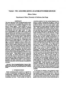
Figure 1: PASS. Step A: A periodic signal can be divided into sinusoidal components. Step B: Computing polynomial coefficients to approximate the signal for each partial. Step C: A polynomial generator is obtained by summing the coefficients from the polynomials of the partials. The values computed by the generator will be the samples of the sound signal.
Measuring the performance of the approach of a signal u(t) by a polynomial U (t) on a validity period p can be done using the SNR ratio given by: Rp 2 u (t)dt R SNR = 10log10 p 0 (u(t) − U (t))2 dt 0 For a given polynomial degree, we propose to find the polynomial coefficients that minimize the value of the denominator of the SNR: Z p (u(t) − U (t))2 dt 0
3. USING POLYNOMIALS Polynomials have been traditionally used in order to model the parameters of the sinusoidal model [10, 11, 12]. Here, we propose to use polynomials to replace the sine function. Our method consists of first calculating a set of polynomial coefficients for each partial. Polynomial values from polynomials computed with these coefficients approximate the signal of the partial on a part of its period. The classic approach would evaluate the polynomial associated to each oscillator, and then sum up the results, which is quite inefficient. The idea is yet to sum the coefficients in a polynomial generator, then to evaluate the resulting polynomial only once. Indeed, summing polynomials leads to another polynomial of the same degree. The sound samples can be computed from this single resulting polynomial, with a fairly low degree – independent of the number of partials to synthesize. The general process is illustrated by Figure 1. 3.1. Partial Approximation The time-domain signal generated by each partial is defined by a sine function. We propose to approximate this function by a polynomial. To get the polynomial coefficients that can approximate any partial of a sound, we decide to first approximate a unit signal u with amplitude a = 1, frequency f = 1, and phase φ = 0, i.e.: u(t) = sin(2πt) We have to choose a part of the period where we will do the approximation. We call this part the validity period p of the polynomial coefficients. Thus, if we approximate a half period of u, then p = 1/2.
These coefficients have to respect other constraints to maintain a piecewise continuity. For example, with a 2-degree polynomial U and p = 1/2, to impose a C 1 continuity, it is sufficient that U (0) = U (1/2) = 0, and the coefficients ai that minimize: 1 2
Z
(sin(2πt) − (a0 + a1 t + a2 t2 ))2 dt
0
are:
8 < a0 = 0 a1 = 240/π 3 : a2 = −480/π 3
To approach the sine function, we can use in this case alternately Ua for a first half period and Ub for the second: Ua (t) = a1 t + a2 t2 Ub (t) = −a1 t − a2 t2 The choice of the validity period, and the highest degree of the polynomials to use, have a big influence on the performance of the approximation, as shown in Table 1. We explain in 3.3 how a high polynomial degree can lead to numerical instability of the method, or in Section 6 why the choice of a short validity period increases the computation time. We can note that using a validity period p = 1/2 with a polynomial degree d = 2 is particularly suited for a very fast synthesis, and that using a validity period p = 1/2 with a polynomial degree d = 4 is suited for a fast synthesis with good quality. The coefficients we compute define a unit polynomial U (t) by validity period. When the unit polynomial is found, every partial can be approximated from it. In the general case of a partial i with
DAFX-182
Proc. of the 9th Int. Conference on Digital Audio Effects (DAFx-06), Montreal, Canada, September 18-20, 2006
amplitude ai , frequency fi , and initial phase φi , the approximating polynomial Pi is then given by: „ « φi Pi (t) = ai U fi t + 2π
hal-00307931, version 1 - 29 Jul 2008
Notice that the amplitude, frequency, or phase parameters do not modify the approximation error given in Table 1. In addition to the sinusoid, the polynomial approximation generates a noise consisting of harmonics of this sinusoid. The magnitudes of these harmonics are small, and depend on the validity period p and the polynomial degree d. p 1/4 1/4 1/4 1/4 1/2 1/2 1/2 1/2 1 1
d 2 3 4 5 2 3 4 5 4 5
C 0 SNR (dB) 36 57 79 102 28 28 59 59 17 42
C 1 SNR (dB) 28 28 59 59 28 28 59 59 17 42
Table 1: Error of polynomial approximation of a partial. For two different continuity requirements (C 0 and C 1 ), the Signal-to-Noise Ratio (SNR) obtained with the approximation error u − U compared to the target signal u are shown as functions of the validity period p and the polynomial degree d.
Since for now we consider only constant parameters for the partials, the generated functions are periodic. It is thus possible to compute the polynomial coefficients for only one period of any partial. Each set of polynomial coefficients is valid for a part of the period of the sine function. For example, if we choose to approximate sine functions using a fourth of their period, we need to compute four sets of coefficients by partial. As long as the amplitude and the frequency of a partial are constant, we can continue with the same pre-calculated sets. During the sound synthesis, the coefficients that approximate the partials must be updated regularly (the rate depending on the frequency of each partial), and must also be changed if the parameters have changed. 3.2. Incremental Calculation of Polynomials To avoid the problem of computing a polynomial with large time values, leading to numerical imprecision, we propose to use the Taylor’s theorem to compute it. The polynomial can be evaluated at every instant t0 + ∆t by using the value and the values of its derivatives at a preceding instant t0 : P k (t0 + ∆t ) = P k (t0 ) +
d X i=k+1
∆i−k t Pi (i − k)!
With the polynomial coefficients of the partials obtained according to the method presented in Section 3.1, we compute the first value of the polynomial and of its derivatives. To compute each of the following values, we use Equation 3 with a step ∆t corresponding to the time between two time events. A time event is either the time of a sound sample or of a scheduled update of the coefficients. When time reaches or exceeds the validity period we have chosen, the coefficients are updated, and the incremental algorithm goes on with the new coefficients. 3.3. Polynomial Generator Using this incremental method for each individual partial would be very expensive in terms of computation time. For that reason, we propose a technique in which we sum the coefficients to compute only a global polynomial, the generator. During the synthesis, the generator is computed incrementally. When a partial reaches the end of its validity period, the different values of the generator (value and values of the derivatives) are summed with the new values from the partial. When a sound sample must be produced, the generator is computed to get the sound sample value. As the generator is computed incrementally, we have to care about numerical precision: using the preceding values to compute new ones accumulates floating-point precision errors in the result. Thus, there is a validity limit for updating the generator. According to the polynomial degree used, to the number of partials in the sound, and the floating-point precision we can use, we need to re-initialize the generator coefficients regularly with the authentic sine function. The complexity of our method is dominated by the management of the update events from individual partials. To optimize this process, we propose the use of an efficient data structure, in a way similar to that of [8] which uses a skip-list to increase the performance of additive synthesis. In the PASS method, we use a priority queue implemented as a binary heap to manage the update events from the partials.
4. DATA STRUCTURE 4.1. Using a Heap as a Priority Queue A priority queue is an abstract data type supporting two operations: insert adds an element to the queue with an associated priority; delete-max removes the element from the queue that has the highest priority, and returns it. We use a priority queue to manage update events from partials of the sound. During synthesis, update events are regularly inserted in, or removed and processed. The standard implementation of priority queues is based on binary heaps (see for example [13]). With this implementation, queue operations have O(log(N )) complexity, with N the number of elements in the queue. A binary heap is a binary tree satisfying two constraints:
(3)
where P k is the k-th derivative of the polynomial function (P 0 being the polynomial itself). The number of necessary values depends on the degree of the polynomial (e.g., three values with a 2-degree polynomial).
DAFX-183
1. the tree is either a perfect binary tree, or, if the last level of the tree is not complete, the nodes are filled from left to right; 2. each node is greater (in priority) than or equal to each of its children. The top of the binary heap is always the next event to process.
Proc. of the 9th Int. Conference on Digital Audio Effects (DAFx-06), Montreal, Canada, September 18-20, 2006
hal-00307931, version 1 - 29 Jul 2008
4.2. Heap Optimization
5. CHANGE OF SOUND PARAMETERS
Most of the computation time of the PASS method is due to the management of the heap. Consequently, heap primitives need to be highly optimized. Our first approach was to delete-max the priority queue, to process the update event and to insert a new one in the queue. With this approach, the heap is substantially reorganized twice for each insert / delete pair of operations. To improve the performance, we replaced the insert / delete primitives with top and replace. top returns the element of the queue that has the highest priority, without removing it. It is possible to process an update event without removing it from the queue. The replace method replaces the element from the queue that has the highest priority with an other element by initially putting it on top of the heap, and then letting it trickle down according to normal heap-reorganization primitives. In the worst case, the replace method needs O(log(N )) operations, N being the number of elements in the heap. The heap is reorganized only once per update. Partials with high frequencies must be updated more often than the others, because their validity period is smaller. With the replace method, the update events concerning high frequencies stay near to the top of the heap. Using fewer operations for the most frequently updates improves the complexity of our method. Figures 2 and 3 give an example of heap management, where the delete-max then insert methods use 4 elements swaps, whereas the replace method takes only 1 swap. 24
8
23
45
36
48
17
72
23
24
45
36
48
48
17
(b)
5
5
17
72
9
22
6
36
23
45
24
6
22
72
(a)
23
45
22
8
36
8
9
.
9
24
48
8
22
(d)
Figure 2: delete-max then insert priority queue methods within a heap. (a) Delete-max of the element with highest priority. (b) Heap reorganization. (c) Insert of the new element. (d) Heap reorganization.
6
5
5
8
36
23
45
48
17
72
(a)
24
6
8
9
22
36
23
45
48
Figure 5: Changing the frequency either when the signal is minimal (left) or maximal (right). It appears that the right case is better, since it avoids derivative discontinuities (clicks).
17
72
(c)
9
Figure 4: Changing the amplitude either when the signal is minimal (left) or maximal (right). It appears that the left case is much better, since it avoids amplitude discontinuities (clicks).
5
5
9
We consider that the parameters of the partials are constant on a short length. But since they change, they have to be updated regularly. In [14] we indicate the best time in a period to change parameters of a partial, as illustrated by Figure 4 and 5. The best moment to change the amplitude is when the signal is minimal, to preserve the continuity of the signal. And the best moment to change the frequency is when the signal is maximal, to preserve the continuity of the signal derivative.
17
72
22
24
Changing parameters of partials with the PASS method consists in changing the polynomial coefficients of an oscillator when this oscillator must be normally updated, because of the end of its validity period. Thus, this change does not need more computation time than without changing the parameters. The best case is with the validity period p = 1/4. In this case we can update the parameters at the best moment we described before for the frequency or the amplitude. Otherwise an update event will be added in the priority queue, to indicate the time to change the parameters of the partials. But few events will be added regarding to the normal updates of the coefficients, and it will not really affect the general computation time. The parameters are updated in the right moment to avoid clicks in the sound. This moment is different for every partials, regarding to their frequencies.
(b)
6. COMPLEXITY AND RESULTS
Figure 3: replace priority queue method with a heap. (a) Replace of the element with highest priority by the new one. (b) Heap reorganization.
The complexity of the PASS method depends on the use of the priority queue. For one second of synthesis, the priority queue will be used f /p times per partial, where p is the validity period chosen (1/2 for a half of a sine period), and f the frequency of the
DAFX-184
Proc. of the 9th Int. Conference on Digital Audio Effects (DAFx-06), Montreal, Canada, September 18-20, 2006
partial. For every partial, the queue operations are called X times per second, where:
hal-00307931, version 1 - 29 Jul 2008
X=
N 1X N f¯ fi = p i=1 p
(4)
with N being the number of partials in the sound, p the validity period, fi the frequency of the partial i, and we denote by f¯ the mean frequency of the partials. If we consider that each priority queue operation is done with O(log(N )) complexity for an update event, with N the number of elements simultaneously in the queue (i.e. the number of partials in the sound), the complexity C1 due to the priority heap managing is given by: „ ¯ « Nf C1 = O log N (5) p We can note that this complexity is very dependent from the mean frequency of the partials. It explains why the method is particularly efficient for low-frequency signals. If the validity period p is doubled (from a fourth to a half of period for example), the performance of the PASS method is doubled too. The higher is p and the better is the complexity of the method. But if we want to increase p, we need to use higher polynomial degree to approximate the sine function. And it leads to numerical instability. We have to find a trade-off between complexity and stability. In addition to C1 is the C2 complexity, to produce the samples of the sound. If we use Fs as the sampling rate and d the polynomial degree of the generator, it is given by: C2 = O(dFs ) Thus, the general complexity of PASS is: „ « N f¯ CPASS = O α log N + dFs p
N 4000 4000 4000
N 2500 2500 2500 2500 5000 5000 5000
(7)
(8)
f¯ 300 300 300
Fs (Hz) 22050 44100 96000
DR 3.2 s 6.3 s 13.7 s
PASS 6.6 s 6.6 s 6.6 s
Table 2: Comparison of the computation time of the Digital Resonator (DR) and PASS methods using different sampling rates, for 5 seconds of sound synthesis, implemented in C language, compiled using the GNU C compiler (gcc) version 4.1, and executed on an Intel Pentium 4 1.8-GHz processor. The PASS method is used with 2-degree polynomials and a validity period p = 1/2. N is the number of partials, f¯ is the mean frequency of the partials, and Fs is the sampling rate.
(6)
where α is some constant which is architecture-dependent (in practice, the synthesis methods were implemented in C language, compiled using the GNU C compiler (gcc) versions 4.0 and 4.1, and executed on PowerPC G4 1.25-GHz and Intel Pentium 4 1.8-GHz processors). This global complexity is a function of the sum of the frequencies of the partials, and we notice that it does not strongly depend on the sample rate anymore. Increasing the sample rate from 44.1 kHz to 96 kHz does not really affect the computation time, as illustrated by Table 2. One might reasonably ask how our method compares to other methods for additive synthesis. Recently, we showed in [7] that the digital resonator method was a little better than the synthesis using the FFT−1 method. But later, Meine an Purnhagen [15] compared different methods and concluded that the fastest additive synthesis is now the FFT−1 method. In fact, this highly depends on the implementation details and computer used, as well as the number of partials and sampling rate. However, the digital resonator easily allows the fine control of each partial of the sound, which is not really the case the FFT−1 method. The PASS method allows the same fine control, and thus we have compared the performance of our method with that of the digital resonator method. And if we have just noted that for PASS method the sample rate does not really affect the computation time, it is not the same with the digital resonator. The complexity CDR of the digital resonator method is given by: CDR = O(N Fs )
with Fs the sampling rate, and N the number of partials in the sound. Here N and Fs are multiplied. This difference of complexity between digital resonator and PASS methods is illustrated by Table 2. As shown in Table 3 or in Figure 6, the method we present is clearly better than the digital resonator for low frequencies. Using a 2-degree polynomial to approximate a half of a period of each partial, PASS is better for 2500 partials when the mean frequency of the partials is under 300 Hz, and even 500 Hz for a 96-kHz sampling rate. Real-time synthesis can be achieved with 5000 partials with a frequency of 150 Hz for example.
f¯ 200 300 400 500 200 300 400
DR 3.9 s 3.9 s 3.9 s 3.9 s 7.9 s 7.9 s 7.9 s
PASS 2.0 s 3.0 s 4.0 s 5.0 s 7.3 s 10.6 s 14.4 s
Table 3: Comparison of the computation time of the Digital Resonator (DR) and PASS methods, for 5 seconds of sound synthesis with a sampling rate of 44100 Hz, implemented in C language, compiled using the GNU C compiler (gcc) version 4.1, and executed on an Intel Pentium 4 1.8-GHz processor. The PASS method is used with 2-degree polynomials and a validity period p = 1/2. N is the number of partials, f¯ is the mean frequency of the partials.
7. CONCLUSION AND FUTURE WORK We have presented PASS, a new additive synthesis method using polynomials. The computation time of this method depends mainly on the sum of the frequencies of the partials. We have shown that the method is fast, and particularly efficient for signals with low frequency partials, as well as for high sampling rates. In the near future, we plan to tune the trade-off between complexity and stability for our method on the fly, by combining the advantages of the PASS and Digital Resonator (DR) methods, since these methods both manipulate oscillators. For this hybrid method, the idea is, for a given partial, to use either PASS or DR depending
DAFX-185
Proc. of the 9th Int. Conference on Digital Audio Effects (DAFx-06), Montreal, Canada, September 18-20, 2006
40
20 PASS DR - 44100 Hz DR - 96000 Hz
30 computation time (s)
15 computation time (s)
PASS DR - 44100 Hz DR - 96000 Hz
35
10
25 20 15 10
5
5 0
100
200
300 400 500 mean frequency (Hz)
600
700
0
800
hal-00307931, version 1 - 29 Jul 2008
(a)
0
1000
2000
3000
4000 5000 6000 number of partials
7000
8000
9000
10000
(b)
Figure 6: Comparison of the computation times of the Digital Resonator (DR) and PASS method, for 5 seconds of sound synthesis. (a) Computation times are functions of the mean frequency f¯, with a fixed number of partials N = 3000. (b) Computation times are functions of the number of partials N , with a fixed mean frequency f¯ = 200 Hz. The PASS method is used with 2-degree polynomials and a validity period p = 1/2. For this comparison, both methods were implemented in C language, compiled using the GNU C compiler (gcc) version 4.0, and executed on a PowerPC G4 1.25-GHz processor.
on the frequency of the partial. For low frequencies, PASS will be preferred. Also, the DR method will take advantage of the priority queue to schedule its optimal update times (see Section 5). At each update time, for the concerned oscillator the decision of switching from PASS to DR or from DR to PASS could be decided. And since at this update time, the amplitude, frequency, and also phase of the oscillator is known, the switch of method is really straightforward. 8. REFERENCES [1] J. A. Moorer, “Signal processing aspects of computer music – a survey,” Computer Music J., vol. 1, no. 1, pp. 4–37, 1977.
[8] M. Lagrange and S. Marchand, “Real-time additive synthesis of sound by taking advantage of psychoacoustics,” in Proc. COST-G6 Conf. on Digital Audio Effects (DAFx-01), Limerick, Ireland, 2001, pp. 5–9. [9] A. Freed, X. Rodet, and P. Depalle, “Synthesis and control of hundreds of sinusoidal partials on a desktop computer without custom hardware,” in Proc. ICSPAT, 1992, pp. 98–101. [10] Y. Ding and X. Qian, “Processing of musical tones using a combined quadratic polynomial-phase sinusoid and residual (QUASAR) signal model,” J. Audio Eng. Soc., vol. 45, no. 7/8, pp. 571–584, 1997.
[2] R. J. McAulay and T. F. Quatieri, “Speech analysis/synthesis based on a sinusoidal representation,” IEEE Trans. Acoust., Speech, and Signal Proc., vol. 34, no. 4, pp. 744–754, 1986.
[11] L. Girin, S. Marchand, J. di Martino, A. Röbel, and G. Peeters, “Comparing the order of a polynomial phase model for the synthesis of quasi-harmonic audio signals,” in Proc. IEEE Workshop Appl. of Dig. Sig. Proc. to Audio and Acoust., New Palz, NY, 2003, pp. 193–196.
[3] X. Serra and J. O. Smith, “Spectral Modeling Synthesis: A sound analysis/synthesis system based on a deterministic plus stochastic decomposition,” Computer Music J., vol. 14, no. 4, pp. 12–24, 1990.
[12] M. Raspaud, S. Marchand, and L. Girin, “A generalized polynomial and sinusoidal model for partial tracking and time stretching,” in Proc. Int. Conf. on Digital Audio Effects (DAFx-05), Madrid, Spain, 2005, pp. 24–29.
[4] J. W. Gordon and J. O. Smith, “A sine generation algorithm for VLSI applications,” in Proc. Int. Comp. Music Conf. (ICMC’85), Burnaby, Canada, 1985, pp. 165–168.
[13] A. V. Aho, J. E. Hopcroft, and J. D. Ullman, Data Structures and Algorithms, ser. Series in Computer Science and Information Processing. Addison-Wesley, 1983, pp. 392–407.
[5] J. O. Smith and P. R. Cook, “The second-order digital waveguide oscillator,” in Proc. Int. Comp. Music Conf. (ICMC’92), San Francisco, USA, 1992, pp. 150–153.
[14] R. Strandh and S. Marchand, “Real-time generation of sound from parameters of additive synthesis,” in Proc. Journées d’Informatique Musicale, 1999, pp. 83–88.
[6] S. Marchand and R. Strandh, “InSpect and ReSpect: Spectral modeling, analysis and real-time synthesis software tools for researchers and composers,” in Proc. Int. Comp. Music Conf. (ICMC’99), Beijing, China, 1999, pp. 341–344.
[15] N. Meine and H. Purnhagen, “Fast sinusoid synthesis for MPEG-4 HILN parametric audio decoding,” in Proc. Int. Conf. on Digital Audio Effects (DAFx-02), Hamburg, Germany, 2002, pp. 239–244.
[7] S. Marchand, “Sound models for computer music (analysis, transformation, and synthesis of musical sound),” Ph.D. dissertation, University of Bordeaux 1, France, 2000.
DAFX-186