Our partials are not strictly sinusoidal, how- ever. We employ a technique of Bandwidth ..... ble to achieve good frequency resolution with shorter (in ..... any pitch may be played, and smooth glissandi are possi- ble. ..... Concord Jazz, Inc., 1994,.
On the Use of Time-Frequency Reassignment in Additive Sound Modeling Kelly Fitz and Lippold Haken
Abstract
(i.e. a model having a single component type) that is capable of representing at high fidelity a wide variety of sounds, including non-harmonic, polyphonic, impulsive, and noisy sounds. The Reassigned Bandwidth-Enhanced Sound Model is robust under transformation, and the fidelity of the representation is preserved even under timedilation and other model-domain modifications. The homogeneity and robustness of the reassigned bandwidthenhanced model make it particularly well-suited for such manipulations as cross synthesis and sound morphing.
We introduce the use of the method of reassignment in sound modeling to produce a sharper, more robust additive representation. The Reassigned BandwidthEnhanced Additive Model follows ridges in a timefrequency analysis to construct partials having both sinusoidal and noise characteristics. This model yields greater resolution in time and frequency than is possible using conventional additive techniques, and better preserves the temporal envelope of transient signals, even in modified reconstruction, without introducing new component types or cumbersome phase interpolation algorithms.
0
Reassigned bandwidth-enhanced modeling and rendering and many kinds of manipulations, including morphing, have been implemented in an open-source C++ class library, Loris, and a stream-based, real time implementation of bandwidth-enhanced synthesis is available in the Symbolic Sound Kyma environment.
Introduction 1
The method of reassignment has been used to sharpen spectrograms to make them more readable [1], to measure sinusoidality, and to ensure optimal window alignment in analysis of musical signals [2]. We use time-frequency reassignment to improve our BandwidthEnhanced Additive Sound Model. The bandwidthenhanced additive representation is similar in spirit to traditional sinusoidal models [3, 4, 5] in that a waveform is modeled as a collection of components, called partials, having time-varying amplitude and frequency envelopes. Our partials are not strictly sinusoidal, however. We employ a technique of Bandwidth Enhancement to combine sinusoidal energy and noise energy into a single partial having time-varying amplitude, frequency, and bandwidth parameters [6, 7]. We use the method of reassignment to improve the time and frequency estimates used to define our partial parameter envelopes, thereby improving the time-frequency resolution of our representation, and improving its phase accuracy.
Time-Frequency Reassignment
The discrete short-time Fourier transform is often used as the basis for a time-frequency representation of timevarying signals, and is defined as a function of time index n and frequency index k as Xn (k) =
∞ X
h(l − n)x(l)e
−j2π(l−n)k N
(1)
l=−∞ N −1 2
=
X
h(l)x(n + l)e
−j2πlk N
(2)
l=− N 2−1
where h(n) is a sliding window function equal to 0 for n < − N 2−1 and n > N 2−1 (for N odd), so that Xn (k) is the N -point discrete Fourier transform (DFT) of a shorttime waveform centered at time n. As a time-frequency representation, the STFT provides relatively poor temporal data. Short-time Fourier data is sampled at a rate equal to the analysis hop size, so data in derivative time-frequency representations is re-
The combination of time-frequency reassignment and bandwidth enhancement yields a homogeneous model 1
In the vicinity of t = τ (i.e., for an analysis window centered at time t = τ ), the point of maximum spectral energy contribution has time-frequency coordinates that satisfy the stationarity conditions
ported on a regular temporal grid, corresponding to the centers of the short-time analysis windows. The sampling of these so-called frame-based representations can be made as dense as desired by an appropriate choice of hop size. Temporal smearing due to the long analysis windows needed to achieve high frequency resolution presents a much more serious problem that cannot be relieved by denser sampling.
∂ [φ (τ, ω) + ω · (t − τ )] = 0 ∂ω ∂ [φ (τ, ω) + ω · (t − τ )] = 0 ∂τ
Though the short-time phase spectrum is known to contain important temporal information, typically, only the short-time magnitude spectrum is considered in the timefrequency representation. The short-time phase spectrum is sometimes used to improve the frequency estimates in the time-frequency representation of quasi-harmonic sounds [8], but it is often omitted entirely, or used only in unmodified reconstruction, as in the Basic Sinusoidal Model, described by McAulay and Quatieri [3].
(3) (4)
where φ (τ, ω) is the continuous short-time phase spectrum and ω · (t − τ ) is the phase travel due to periodic oscillation [9]. The stationarity conditions are satisfied at the coordinates ∂φ (τ, ω) tˆ = τ − ∂ω ∂φ (τ, ω) ω ˆ = ∂τ
It has been shown that partial derivatives of the shorttime phase spectrum can be used to substantially improve the short-time time and frequency resolution [9], and an efficient short-time Fourier transform-based implementation has been developed that does not require complex division [1].
(5) (6)
representing, respectively, the group delay and instantaneous frequency. Discretizing Equations (5) and (6) to compute the time and frequency coordinates numerically is difficult and unreliable, because the partial derivatives must be approximated. These formulae can be rewritten in the form of ratios of discrete Fourier transforms [1]. Time and frequency coordinates can be computed using two additional short-time Fourier transforms, one employing a time-weighted window function and one employing a frequency-weighted window function.
The so-called Method of Reassignment computes reassigned time and frequency estimates for each spectral component from partial derivatives of the short-time phase spectrum. Instead of locating time-frequency components at the geometrical center of the analysis window (tn , ωk ), as in traditional short-time spectral analysis, the components are reassigned to the center of gravity of their complex spectral energy distribution, computed from the short-time phase spectrum according to the principle of stationary phase. This method was first developed in the context of the spectrogram and called the Modified Moving Window Method [9], but has since been applied to a variety of time-frequency and timescale transforms [1].
Since time estimates correspond to the temporal center of the short-time analysis window, the time-weighted window is computed by scaling the analysis window function by a time ramp the time ramp from − N 2−1 to N 2−1 , for a window of length N . The frequency-weighted window is computed by wrapping the Fourier transform of the analysis window to the frequency range [−π, π], scaling the transform by a frequency ramp from − N 2−1 to N −1 2 , and inverting the scaled tranform to obtain a (real) frequency-scaled window. Using these weighted windows, the method of reassignment computes corrections to the time and frequency estimates in fractional sample units between − N 2−1 and N 2−1 . The three analysis windows employed in reassigned short-time Fourier analysis are shown in Figure 1.
The theorem of stationary phase states that the variation of the Fourier phase spectrum not attributable to periodic oscillation is slow with respect to frequency in certain spectral regions, and in surrounding regions the variation is relatively rapid. In Fourier reconstruction, positive and negative contributions to the waveform cancel in frequency regions of rapid phase variation. Only regions of slow phase variation (stationary phase) will contribute significantly to the reconstruction, and the maximum contribution (center of gravity) occurs at the point where the phase is changing most slowly with respect to time and frequency.
The method of reassignment computes reassigned times a frequencies for each short-time spectral component. The reassigned time, tˆk,n , for the k th spectral component from the short-time analysis window centered at time n (in samples, assuming odd-length analysis win2
Analysis windows used in time−frequency reassignment
in the representation is relocated by a process that is highly signal dependent. This is not an issue in our representation, since the bandwidth-enhanced additive model, like the basic sinusoidal model [3], retains data only at time-frequency ridges (peaks in the short-time magnitude spectra), and thus is not bilinear.
1 h(n)
0.8 0.6 0.4 0.2 −250
−200
−150
−100
−50
0 n
50
100
150
200
250
40 ht(n)
20 0
Note that, since the short-time Fourier transform is invertible, and the original waveform can be exactly reconstructed from an adequately-sampled short-time Fourier representation, all the information needed to precisely locate a spectral component within an analysis window is present in the short-time coefficients, Xn (k). Temporal information is encoded in the short-time phase spectrum, which is very difficult to interpret. The method of reassignment is a technique for extracting information from the phase spectrum.
−20 −40 −250
−200
−150
−100
−50
0 n
50
100
150
200
250
−200
−150
−100
−50
0 n
50
100
150
200
250
f
h (n)
100 0
−100 −250
Figure 1: Analysis windows employed in the three shorttime transforms used to compute reassigned times and frequencies. Waveform (a) is the original window function, h (n) (a 501 point Kaiser window with shaping parameter 12.0, in this case), waveform (b) is timeweighted window function, ht (n) = n h (n), and waveform (c) is the frequency-weighted window function, hf (n).
2
(
Xt;n (k)Xn∗ (k) 2
|Xn (k)|
Bandwidth-
The method of reassignment has been used to sharpen spectrograms to make them more readable [1, 10]. We use it to improve our bandwidth-enhanced sinusoidal modeling representation [6, 7]. The Reassigned Bandwidth-Enhanced Additive Model [11] employs time-frequency reassignment to improve the time and frequency estimates used to define our partial parameter envelopes, thereby improving the time-frequency resolution of our representation, and improving its phase accuracy.
dows) is [1] tˆk,n = n −
0
(10)
The bandwidth-enhanced oscillator is depicted in Figure 2.
3
We define the time-varying bandwidth coefficient, κ(n), as the fraction of total instantaneous partial energy that is attributable to noise. This bandwidth (or noisiness) coefficient assumes values between 0 for a pure sinusoid and 1 for partial that is entirely narrowband noise, and varies over time according to the noisiness of the partial. If we represent the total (sinusoidal and noise) instantaneous partial energy as A˜2 (n), then the output of the bandwidth-enhanced oscillator is described by hp i p ˜ y(n) = A(n) 1 − κ(n) + 2κ(n)ζ(n) cos (θ(n)) (11)
Sharpening Transients
Time-frequency representations based on traditional magnitude-only short-time Fourier analysis techniques (such as the spectrogram and the basic sinusoidal model [3]) fail to distinguish transient components from sustaining components. A strong transient waveform, as shown in Figure 4a, is represented by a collection of low amplitude spectral components in early short-time analysis frames, that is, frames corresponding to analysis windows centered earlier than the time of the transient. A low-amplitude periodic waveform, as shown in Figure 4b, is also represented by a collection of low amplitude spectral components. The information needed to distinguish these two critically different waveforms is encoded in the short-time phase spectrum, and is extracted by the method of reassignment.
The envelopes for the time-varying partial amplitudes and frequencies are constructed by identifying and following ridges on the time-frequency surface. The timevarying partial bandwidth coefficients are computed and assigned by a process of bandwidth association [6].
Other methods have been proposed for representing transient waveforms in additive sound models. Verma and Meng [12] introduce new component types specifically for modeling transients, but this method sacrifices the ho-
We use the method of reassignment to improve the time 4
ω8
ω7
ω7
ω7
ω6
ω6
ω6
ω5 ω4 ω3
Frequency
ω8
Frequency
Frequency
ω8
ω5 ω4 ω3
ω5 ω4 ω3
ω2
ω2
ω2
ω1
ω1
ω1
t1
t2
t3
t4
t5
t6
t1
t7
t2
t3
t4
Time
Time (a)
(b)
t5
t6
t7
t1
t2
t3
t4
t5
t6
t7
Time (c)
Figure 3: Comparison of time-frequency data included in common representations. Only the time-frequency orientation of the data points is shown. The short-time Fourier transform (a) retains data at every time tn and frequency ωk . The basic sinusoidal model [3] retains data at selected time and frequency samples, as shown in (b). Reassigned bandwidth-enhanced analysis data (c) is distributed continuously in time and frequency, and retained only at timefrequency ridges. Arrows indicate the mapping of short-time spectral samples onto time-frequency ridges due to the method of reassignment. mogeneity of the model. A homogeneous model, that is, a model having a single component type, such as the breakpoint parameter envelopes in our reassigned bandwidth-enhanced additive model [11], is critical for many kinds of manipulations [13, 14]. Peeters and Rodet [2] have developed a hybrid analysis/synthesis system that eschews high-level transient models and retains unabridged OLA (overlap-add) frame data at transient positions. This hybrid representation represents unmodified transients perfectly, but also sacrifices homogenity. Quatieri [15] proposes a method for preserving the temporal envelope short-duration complex acoustic signals using a homogeneous sinsusoidal model, but it is inapplicable to longer duration sounds, or sounds having multiple transient events.
1 0.8 0.6 0.4 0.2 0 −0.2
0
100
200
300
400
500
600
700
400
500
600
700
time
1 0.8 0.6 0.4 0.2 0 −0.2
0
100
200
300
Time-frequency reassignment allows us to preserve temporal envelope shape without sacrificing the homogeneity of the bandwidth-enhanced additive model. Reassignment greatly improves time resolution by relocating spectral peaks closer to the time of the transient events, so that transients are not smeared out by the length of the analysis window. Components extracted from early or late short-time analysis windows are reassigned to times near the time of the transient, yielding clusters of time-frequency data points, as shown in the reassigned analysis depicted in Figure 3. Moreover, since reassignment sharpens our frequency estimates, it is possible to achieve good frequency resolution with shorter (in time) analysis windows than would be possible with traditional methods. The use of shorter analysis windows
time
Figure 4: Two windowed short-time waveforms (dashed lines) that are not readily distinguished in the basic sinsoidal model [3]. Both waveforms are represented by low-amplitude spectral components, and with reassignment, the strong transient on the left (a) yields off-center components, having large time corrections (positive in this case because the transient is near the right tail of the window), while the sustained quasi-periodic waveform on the right (b) yields time corrections near zero.
5
out by the long analysis window. Figure 7 shows a reconstruction from reassigned time-frequency data. The transient response has been greatly improved by relocating components extracted from early analysis windows (like the one on the left in Figure 5) to their spectral centers of gravity, closer to the observed turn-on time. The synthesized onset time has been reduced to approximately 10 ms. The time-frequency analysis data is shown in Figure 8. The nonreassigned data is evenly distributed in time, so data from early windows (that is, windows centered before the onset time) smears the onset, whereas the reassigned data from early analysis windows is clumped near the correct onset time.
Amplitude
1
0
−1 60
310 Time
Figure 5: Two long analysis windows superimposed at different times on a square wave signal with an abrupt turn-on. The short-time transform corresponding to the earlier window generates unreliable parameter estimates and smears the sharp onset of the square wave.
4
Cropping
Off-center components are short-time spectral components having large time reassignments, that is, components having centers of gravity far from the temporal center of the analysis window. Since they represent transient events that are far from the center of the analysis window, and are therefore poorly represented in the windowed short-time waveform, these off-center components introduce unreliable spectral parameter estimates that corrupt our representation, making the model data difficult to interpret and manipulate.
further improves our time resolution and reduces temporal smearing. The effect of time-frequency reassignment on transient response can be demonstrated using a square wave that turns on abruptly, shown in Figure 5. This waveform, while aurally uninteresting and uninformative, is useful for visualizing the performance of various analysis methods. Its abrupt onset makes temporal smearing obvious, its simple harmonic partial amplitude relationship makes it easy to predict the necessary data for a good time-frequency representation, and its simple waveshape makes phase errors and temporal distortion easy to identify. Note, however, that this waveform is pathological for Fourier-based additive models, and exaggerates all of these problems with such methods. We use it only for comparison of various methods. Figures 6 and 7 show two reconstructions of the onset of the square wave in Figure 5 from time-frequency data obtained using a 54-ms analysis window. The silence before the onset is not shown. Only the first (lowest frequency) five harmonic partials were used in the reconstruction, and consequently the ringing due to Gibb’s phenomenon is evident.
Fortunately, large time corrections make off-center components easy to identify and remove from our model. By removing the unreliable data embodied by off-center components, we make our model cleaner and more robust. Moreover, thanks to the redundancy inherent in short-time analysis with overlapping analysis windows, we do not sacrifice information by removing the unreliable data points. The information represented poorly in off-center components is more reliably represented in well-centered components, extracted from analysis windows centered nearer the time of the transient event. Figure 9 shows reassigned bandwidth-enhanced model data from the onset of a bowed cello tone before and after the removal of off-center components. Typically, data having time corrections greater than the time between consecutive analysis window centers is considered to be unreliable, and is removed, or cropped.
Figure 6 is a reconstruction from traditional, nonreassigned time-frequency data. The reconstructed square wave amplitude rises very gradually and reaches full amplitude approximately 40 ms after the first non-zero sample. Clearly, the instantaneous turn-on has been smeared
Cropping partials to remove off-center components allows us to localize transient events reliably. Figure 8(c) shows reassigned time-frequency data from the abrupt square wave onset with off-center components removed. The abrupt square wave onset synthesized from the 6
Amplitude
Time (ms)
22
22
Time (ms)
44
Amplitude
0
Amplitude
Figure 6: Onset of square wave reconstruction without reassignment.
0
22
Time (ms) Figure 7: Onset of square wave reconstruction with reassignment.
0
0
Time (ms) (a)
60
0
Frequency (Hz)
2000
Frequency (Hz)
2000
Frequency (Hz)
2000
0
Time (ms) (b )
60
0
0
Time (ms) (c)
60
Figure 8: Time-frequency analysis data points for an abrupt square wave onset, depicted in Figure 5. The traditional nonreassigned data (a) is evenly distributed in time, whereas the reassigned data (b) is clumped at the onset time. (c) shows the reassigned analysis data after far off-center components have been removed, or “cropped”. Only time and frequency information is plotted, amplitude information is not displayed.
7
1200 Frequency (Hz)
unmodified reconstruction. In order to match short-time spectral frequency and phase estimates at frame boundaries, McAulay and Quatieri employ cubic interpolation of the instantaneous partial phase.
370
0
Time (ms) (a)
140
0
Time (ms) (b)
140
Cubic phase envelopes have many undesirable properties. They are difficult to manipulate and maintain under time- and frequency-scale transformation compared to linear frequency envelopes. However, in unmodified reconstruction, cubic interpolation prevents the propagation of phase errors introduced by unreliable parameter estimates, maintaining phase accuracy in transients, where the temporal envelope is important, and throughout the reconstructed waveform. The effect of phase errors in unmodified reconstruction of a square wave is illustrated in Figure 11. If not corrected using a technique like cubic phase interpolation, partial parameter errors introduced by off-center components render the wave shape visually unrecognizable. Figure 12 shows that cubic phase can be used to correct these errors in unmodified reconstruction. It should be noted that in this case, the phase errors appear dramatic, but are not important to the sound of the reconstructed waveform. In many sounds, particularly transient sounds, preservation of the temporal envelope is critical [15, 12], but the square waveforms in Figures 11 and 12 sound identical. It should also be noted that cubic phase interpolation can be used to preserve phase accuracy, but does not reduce temporal smearing due to off-center components in long analysis windows.
Frequency (Hz)
1200
370
Figure 9: Time-frequency coordinates of data from reassigned bandwidth-enhanced analysis before (a) and after (b) cropping of off-center components clumped together at partial onsets. The source waveform is a bowed cello tone. cropped reassigned data, seen in Figure 10, is much sharper than the uncropped, reassigned reconstruction, because the taper of the analysis window makes even the time correction data unreliable in components that are very far off-center. Figure 9 shows reassigned bandwidth-enhanced model data from the onset of a bowed cello tone before and after the removal of offcenter components. In this case, components with time corrections greater than 10 milliseconds (the time between consecutive analysis windows) were deemed to be too far off-center to deliver reliable parameter estimates. As in Figure 8(c), the unreliable data clustered at the time of the onset is removed, leaving a cleaner, more robust representation.
5
It is not desirable to preserve phase at all times in modified reconstruction. Because frequency is the time derivative of phase, any change in the time or frequency scale of a partial must correspond to a change in the phase values at the parameter envelope breakpoints. In general, preserving phase using the cubic phase method in the presence of modifications (or estimation errors) introduces wild frequency excursions [16]. Phase can be preserved at one time, however, and that time is typically chosen to be the onset of each partial, although any single time could be chosen. The partial phase at all other times is modified to reflect the new time-frequency characteristic of the modified partial.
Phase Maintenance
Off-center components with unreliable parameter estimates introduce phase errors in modified reconstruction. If the phase is maintained at the partial onset, even the cubic interpolation scheme cannot prevent phase errors from propagating in modified syntheses. This effect is illustrated in Figure 13, in which the square wave timefrequency data has been shifted in frequency by 10% and
Preserving phase is important for reproducing some classes of sounds, particularly transients and shortduration complex audio events having significant information in the temporal envelope [15]. The basic sinusoidal model proposed by McAulay and Quatieri [3] is phase correct, that is, it preserves phase at all times in 8
Amplitude 0
Time (ms)
22
Figure 10: Onset of square wave reconstruction with reassignment and removal of unreliable partial parameter estimates.
6
reconstructed using cubic phase curves modified to reflect the frequency shift. By removing the off-center components at the onset of a partial, we not only remove the primary source of phase errors, we also improve the shape of the temporal envelope in modified reconstruction of transients by preserving a more reliable phase estimate at a time closer to the time of transient event. We can therefore maintain phase accuracy at critical parts of the audio waveform even under transformation, and even using linear frequency envelopes, which are much simpler to compute, interpret, edit, and maintain than cubic phase curves. Figure 14 shows a square wave reconstruction from cropped reassigned time-frequency data, and Figure 15 shows a frequency-shifted reconstruction, both using linear frequency interpolation. Removing components with large time corrections preserves phase in modified and unmodified reconstruction, and thus obviates cubic phase interpolation.
Breaking partials at Transient Events
Transients corresponding to the onset of all associated partials are preserved in our model by removing offcenter components at the ends of partials. If transients always correspond to the onset of associated partials, then that method will preserve the temporal envelope of multiple transient events. In fact, however, partials often span transients. Figure 16 shows a partial that extends over transient boundaries in a representation of a bongo roll, a sequence of very short transient events. The approximate attack times are indicated by dashed vertical lines. In such cases, it is not possible to preserve the phase at the locations of multiple transients, since, under modification the phase can only be preserved at one time in the life of a partial. Strong transients are identified by the large time corrections they introduce. By breaking partials at components having large time corrections, we cause all associated partials to be born at the time of the transient, and thereby enhance our ability to maintain phase accuracy. In Figure 17, the partial that spanned several transients in Figure 16 has been broken at components having time corrections greater than the time between successive analysis window centers (about 1.3 milliseconds, in this case), allowing us to maintain the partial phases at each bongo strike. By breaking partials at the locations of transients, we can preserve the temporal envelope of multiple transient events, even under transformation.
Moreover, since we do not rely on frequent cubic phase corrections to our frequency estimates to preserve the shape of the temporal envelope (which would otherwise be corrupted by errors introduced by unreliable data), we have found that we can obtain very good-quality reconstruction, even under modification, with regularlysampled partial parameter envelopes. That is, we can sample the frequency, amplitude, and bandwidth envelopes of our reassigned bandwidth-enhanced partials at regular intervals (of, for example, 8 milliseconds) without sacrificing the fidelity of the model. We thereby achieve the data regularity of frame-based additive model data and the fidelity of reassigned spectral data. Resampling of the partial parameter envelopes is especially useful in real-time synthesis applications [13, 14].
Figure 18 shows the waveform for two strikes in a bongo roll reconstructed from reassigned bandwidth-enhanced data. The same two bongo strikes reconstructed from nonreassigned data are shown in Figure 19. Comparison to the source waveform shown in Figure 20 reveals that 9
Amplitude 60
Time (ms)
84
Amplitude
Figure 11: Reconstructed square waveform from five harmonic partials using linear frequency interpolation without time-frequency reassignment or removal of off-center components. The 24 ms plot spans slightly less than five periods of the 200 Hz waveform.
60
Time (ms)
84
Amplitude
Figure 12: Reconstructed square waveform from five harmonic partials without time-frequency reassignment or removal of off-center components using cubic phase interpolation, as proposed by McAulay and Quatieri [3].
60
Time (ms)
84
Amplitude
Figure 13: Reconstructed square waveform from five harmonic partials shifted in frequency by 10%, using cubic phase interpolation without time-frequency reassignment or removal of off-center components. Notice that more periods of the (distorted) waveform are spanned by the 24 ms plot than by the plots of unmodified reconstructions, due to the frequency shift.
60
Time (ms)
84
Figure 14: Reconstructed square waveform from five harmonic partials using linear frequency interpolation with timefrequency reassignment and removal of off-center components. 10
Amplitude 60
84
Time (ms)
Figure 15: Reconstructed square waveform from five harmonic partials shifted in frequency by 10%, using linear frequency interpolation with time-frequency reassignment and removal of off-center components. Notice that more periods of the (distorted) waveform are spanned by the 24-ms plot than by the plots of unmodified reconstructions, and that no distortion of the waveform is evident.
2114 2114
Frequnecy (Hz)
1976
Frequnecy (Hz)
1976
1839
1839
1701
1701 1563 1563
1425 0.123
1425 0.123 0.146
0.169
0.193
Time (seconds)
0.216
0.239
0.146
0.170
0.193
Time (seconds)
0.216
0.239
Figure 17: Time-frequency plot of reassigned bandwidth-enhanced analysis data for one strike in a bongo roll with partials broken at components having large time corrections, and far off-center components removed. Dashed vertical lines show the approximate locations of attack transients. Partials break at transient boundaries. Only the time-frequency coordinates of partial data are shown; partial amplitudes are not indicated in this plot.
Figure 16: Time-frequency plot of reassigned bandwidth-enhanced analysis data for one strike in a bongo roll. Dashed vertical lines show the approximate locations of attack transients. The lower-frequency partial extends across transient boundaries. Only the time-frequency coordinates of partial data are shown; partial amplitudes are not indicated in this plot.
11
the reconstruction from reassigned data is better able to preserve the temporal envelope than the reconstruction from nonreassigned data and suffers less from temporal smearing.
stream from the envelope parameter stream. Our real-time synthesis element implements bandwidthenhanced oscillators [7] with the sum y(n)
7
=
K−1 X
[Ak (n) + Nk (n)b(n)] sin θk (n)(12)
k=0
Real–Time Synthesis
θk (n)
= θk (n − 1) + 2Fk (n)
(13)
where Together with Kurt Hebel of Symbolic Sound Corporation, we have implemented a real-time reassigned bandwidth-enhanced synthesizer using the Kyma Sound Design Workstation [17].
• y is the time domain waveform for the synthesized sound,
Many real-time synthesis systems allow the sound designer to manipulate streams of samples. In our realtime reassigned bandwidth-enhanced implementation, we work with streams of data that are not time-domain samples. Rather, our Envelope Parameter Streams encode frequency, amplitude, and bandwidth envelope parameters for each bandwidth-enhanced partial [13, 14].
• n is the sample number,
Much of the strength of systems that operate on sample streams is derived from the uniformity of the data. This homogeneity gives the sound designer great flexibility with a few general-purpose processing elements. In our encoding of envelope parameter streams, data homogeneity is also of prime importance. The envelope parameters for all the partials in a sound are encoded sequentially. Typically, the stream has a block size of 128 samples, which means the parameters for each partial are updated every 128 samples, or 2.9 ms at a 44.1 kHz sampling rate. Sample streams generally do not have block sizes associated with them, but this structure is necessary in our envelope parameter stream implementation. The envelope parameter stream encodes envelope information for a single partial at each sample time, and a block of samples provides updated envelope information for all the partials.
• Nk is partial k’s noise envelope,
Values for the envelopes Ak , Nk , and Fk are updated from the parameter stream every 2.9 ms. The synthesis element performs sample-level linear interpolation between updates, so that Ak , Nk , and Fk are piecewise linear envelopes with 2.9 ms linear segments [18]. The θk values are initialized at partial onsets (when Ak and Nk are zero) from the phase envelope in the partial’s parameter stream.
Envelope parameter streams are usually created by traversing a file containing frame-based data from an analysis of a source recording. Such a file can be derived from a reassigned bandwidth-enhanced analysis by resampling the envelopes at 2.9 ms intervals. The parameter streams may also be generated by real-time analysis, or by real-time algorithms, but that process is beyond the scope of this discussion. A parameter stream typically passes through several processing elements. These processing elements can combine multiple streams in a variety of ways, and can modify values within a stream. Finally, a synthesis element computes an audio sample
Rather than use a separate model to represent noise in our sounds, we use the envelope Nk (in addition to the traditional Ak and Fk envelopes) and retain a homogenous data stream. Quasi-harmonic sounds, even those with noisy attacks, have one partial per harmonic in our representation. The noise envelopes allow a sound designer to manipulate noise-like components of sound in an intuitive way, using a familiar set of controls. We have implemented a wide variety of real-time manipulations on envelope parameter streams, including frequency shifting, formant shifting, time dilation, cross synthesis, and sound morphing.
• k is the partial number in the sound, • K is the total number of partials in the sound (usually between 20 and 160), • Ak is partial k’s amplitude envelope,
• b is a zero-mean noise modulator with bell-shaped spectrum, • Fk is partial k’s log (base 2) frequency envelope, • θk is the running phase for the kth partial.
12
Amplitude 0.14
Time (s)
0.25
Amplitude
Figure 18: Waveform plot for two strikes in a bongo roll reconstructed from reassigned bandwidth-enhanced data.
0.14
Time (s)
0.25
Amplitude
Figure 19: Waveform plot for two strikes in a bongo roll reconstructed from nonreassigned bandwidth-enhanced data, synthesized using cubic phase interpolation to maintain phase accuracy.
0.14
Time (s)
0.25
Figure 20: Plot of the source waveform for the bongo strikes analyzed and reconstructed in Figures 18 and 19.
13
Our new MIDI controller, the Continuum Fingerboard, allows continuous control over each note in a performance. It resembles a traditional keyboard in that it is approximately the same size and is played with ten fingers [14]. Like keyboards supporting MIDI’s polyphonic aftertouch, it continually measures each finger’s pressure. The Continuum Fingerboard also resembles a fretless string instrument in that it has no discrete pitches; any pitch may be played, and smooth glissandi are possible. It tracks the x, y, z position for each finger pressing on the playing surface. These continuous 3-dimensional outputs are a convenient source of control parameters for real-time manipulations on envelope parameter streams.
not intended to constitute proof of the efficacy of our algorithms, or the utility of our representation. They are intended only to illustrate features of some of the sounds used and generated in our experiments. The results of our work can only be judged by auditory evaluation, and to that end, these sounds and many others are available for audition at the Loris web site, www.cerlsoundgroup.org/Loris. All sounds used in these experiments were sampled at 44.1 kHz (CD quality), so time-frequency analysis data is available at frequencies as high as 22.05 kHz. However, for clarity, only a limited frequency range is plotted in most cases. Spectrogram plots all have high gain so that low-amplitude high-frequency partials are visible. Consequently, strong low-frequency partials are very often clipped, and appear to have unnaturally flat amplitude envelopes.
8 Conclusions
Waveform and spectrogram plots were produced using Alberto Ricci’s SoundMaker software application [20]. Plots of sinusoidal and bandwidth-enhanced analysis data were produced using unreleased development versions of the Loris software application [19]. In plots of bandwidth-enhanced analysis data, partial center frequencies are plotted against time, and partial amplitude is indicated by grayscale, with darker lines corresponding to higher amplitude. Partial bandwidth is not indicated on these plots.
The reassigned bandwidth-enhanced additive sound model [11] combines bandwidth-enhanced analysis and synthesis techiniques [6, 7] with the time-frequency reassignment technique described in this paper. We have found that the method of reassignment dramatically strengthens our bandwidth-enhanced additive sound model. Temporal smearing is greatly reduced because the time-frequency orientation of the model data is waveform-dependent, rather than analysis-dependent as in traditional short-time analysis methods. Moreover, time-frequency reassignment allows us to identify unreliable data points (having bad parameter estimates) and remove them from the representation. This not only sharpens the representation and makes it more robust, but it also allows us to maintain phase accuracy at transients, even under transformation, while avoiding the problems associated with cubic phase interpolation.
A
A.1 Flute Tone A flute tone, played at pitch D4 (D above middle C), having a fundamental frequency of approximately 293 Hz and no vibrato, taken from the McGill University Master Samples compact discs [21, Disc 2 Track 1 Index 3] is shown in the 3D spectrogram plot in Figure 21. This sound was modeled by reassigned bandwidth-enhanced analysis data produced using a 53 ms Kaiser analysis window with 90 dB sidelobe rejection. The partials were constrained to be separated by at least 250 Hz, slightly greater than 85% of the harmonic partial separation. Breath noise is a significant component of this sound. This noise is visible between the strong harmonic components in the spectrogram plot, particularly at frequencies above 3 kHz. The breath noise is faithfully represented in the reassigned bandwidth-enhanced analysis data, and reproduced in the reconstructions from that analysis data. A 3D spectrogram plot of the reconstruction is shown in Figure 22. The absence of the breath noise is apparent in spectral plot for sinusoidal recon-
Results
The reassigned bandwidth-enhanced additive model is implemented in the open source C++ class library Loris [19], and is the basis of the sound manipulation and morphing algorithms implemented therein. We have attempted to use a wide variety of sounds in the experiments we conducted during the development of the reassigned bandwidth-enhanced additive sound model. The results from a few of those experiments are presented in this section. Data and waveform plots are 14
struction from non-bandwidth-enhanced analysis data, shown in Figure 23.
A.2
a 71 ms Kaiser window in this case, can degrade the representation. The reconstructed tone plotted in Figure 25 is recognizable, but completely lacks the flutter effect, which has been smeared by the window duration. In this case, multiple transient events are spanned by a single analysis window, and the temporal center of gravity for that window lies somewhere between the transient events. Time-frequency reassignment allows us to identify multiple transient events in a single sound, but not within a single short-time analysis window.
Cello Tone
A cello tone, played at pitch D sharp 3 (D sharp below middle C), having a fundamental frequency of approximately 156 Hz, played by Edwin Tellman and recorded by Patrick Wolfe [22] was modeled by reassigned bandwidth-enhanced analysis data produced using a 71 ms Kaiser analysis window with 80 dB sidelobe rejection. The partials were constrained to be separated by at least 135 Hz, slightly greater than 85% of the harmonic partial separation. Bow noise is a strong component of the cello tone, especially in the attack portion. As with the flute tone, the noise is visible between the strong harmonic components in spectral plots, and was preserved in the reconstructions from reassigned bandwidth-enhanced analysis data and absent from sinusoidal (non-bandwidth-enhanced) reconstructions. Unlike the flute tone, the cello tone has an abrupt attack, which is smeared out in non-reassigned sinusoidal analyses (data from reassigned and non-reassigned cello analysis was plotted in Figure 9), causing the reconstructed cello tone to have weak-sounding articulation. The characteristic “grunt” is much better-preserved in reassigned model data.
A.3
A.4 Bongo Roll Figure 26 shows the waveform and spectrogram for an 18-strike bongo roll taken from the McGill University Master Samples compact discs [21, Disc 3 Track 11 Index 31]. This sound was modeled by reassigned bandwidth-enhanced analysis data produced using a 10 ms Kaiser analysis window with 90 dB sidelobe rejection. The partials were constrained to be separated by at least 300 Hz. The sharp attacks in this sound were preserved using reassigned analysis data, but smeared in nonreassigned reconstruction, as discussed in Section 6. The waveforms for two bongo strikes are shown in reassigned and nonreassigned reconstruction in Figures 17 and 16, respectively. Inspection of the waveforms reveals that the attacks in the non-reassigned reconstruction are not as sharp as in the original or the reassigned reconstruction, a clearly audible difference.
Flutter-Tongued Flute Tone
Transient smearing is particularly apparent in timedilated synthesis, where the nonreassigned reconstruction loses the percussive character of the bongo strikes. The reassigned data provides a much more robust representation of the attack transients, retaining the percussive character of the bongo roll under a variety of transformations, including time dilation.
A flutter-tongued flute tone, played at pitch E4 (E above middle C), having a fundamental frequency of approximately 330 Hz, taken from the McGill University Master Samples compact discs [21, Disc 2 Track 2 Index 5] was represented by reassigned bandwidth-enhanced analysis data produced using a 17.8 ms Kaiser analysis window with 80 dB sidelobe rejection. The partials were constrained to be separated by at least 300 Hz, slightly greater than 90% of the harmonic partial separation. The flutter-tongue effect introduces a modulation with a period of approximately 35 ms, and gives the appearance of vertical stripes on the strong harmonic partials in the spectrogram shown in Figure 24.
A.5 Orchestral Gong Figure 27 shows a 3D spectrogram for a strike of an orchestral gong taken from the McGill University Master Samples compact discs [21, Disc 3 Track 12 Index 7]. This sound is very noise-like in the attack, but also has stable, sustained frequency components, visible as long, slowly decaying ridges in the spectrogram, that give the gong a pitched character.
With careful choice of window parameters, reconstruction from reassigned bandwidth-enhanced analysis data preserves the flutter-tongue effect, even under time dilation, and is difficult to distinguish from the original. Figure 25 shows how poor choice of analysis window, 15
Figure 21: 3D spectrogram plot for a breathy flute tone, pitch D4 (D above middle C). Audible low-frequency noise and rumble from the recording is visible. Strong low-frequency components are clipped and appear to have unnaturally flat amplitude envelopes due to the high gain used to make low-amplitude high-frequency partials visible.
Figure 22: 3D spectrogram plot for a breathy flute tone, pitch D4 (D above middle C), reconstructed from reassigned bandwidth-enhanced analysis data.
16
Figure 23: 3D spectrogram plot for a breathy flute tone, pitch D4 (D above middle C), reconstructed from reassigned non-bandwidth-enhanced analysis data. The gong strike is also characterized by the lowfrequency “thud” of the mallet impact, which we were unable to capture without resorting to very long analysis windows that introduced many other artifacts. Analysis of sounds with substantial energy at very low frequencies continues to be difficult because very long windows are needed to accurately estimate the parameters of lowfrequency partials.
phrase span the pitches G3 (G below middle C, approximately 196 Hz fundamental frequency) to B flat 4 (B flat above middle C, approximately 466 Hz fundamental frequency), and a wide range of dynamics. The phrase is divided into five legato subphrases (of three, three, five, four, and three notes, respectively), each having a sharp, tongued attack on the first note. The saxophone phrase was modeled by reassigned bandwidth-enhanced analysis data produced using a 45 ms Kaiser analysis window with 90 dB sidelobe rejection. The partials were constrained to be separated by at least 90 Hz, less than 50% of the harmonic partial spacing for the lowest pitch in the phrase. The narrow partial spacing is necessary to allow the notes to reverberate without being truncated at the next attack.
The gong was modeled by reassigned bandwidthenhanced analysis data produced using a 105 ms Kaiser analysis window with 90 dB sidelobe rejection. The partials were constrained to be separated by at least 25 Hz. The volume of data is very large, due to the small partial spacing. In this case, our representation may not be superior to the sinusoidal representation, although the reconstruction fidelity is higher. However, we were able to reduce the volume of data by approximately one third by pruning the shortest partials (having duration less than 100 ms) from the analysis data and redistributing their energy as noise among neighboring partials without degrading the reconstruction.
A.6
Reconstructions from non-bandwidth-enhanced data lack the ambience of the original, an audible effect not clearly visible in waveform or spectrum plots. The tongued attacks at the first note of each subphrase are smeared in reconstructions from nonreassigned analysis data.
Alto Saxophone Phrase A.7 Piano and Soprano Saxophone Duet
Figure 28 shows the waveform and spectrogram for a mildly ambient recording of a solo alto saxophone phrase played by C. Potter [23]. The nineteen notes in the
An excerpt from a recording of a duet played by J. Lovano, soprano saxophone, and G. Rubalcaba, piano [24], 17
6
Frequency (kHz)
4
2
0
Time (s)
6.7
Amplitude
0
0
Time (s)
6.7
Figure 24: Waveform and spectrogram plot for a flutter-tongued flute tone, pitch E4 (E above middle C). Vertical stripes on the strong harmonic partials indicate modulation due to the flutter-tongue effect. Strong low-frequency components are clipped and appear to have unnaturally flat amplitude envelopes due to the high gain used to make low-amplitude high-frequency partials visible.
18
6
Frequency (kHz)
4
2
0
Time (s)
6.7
Amplitude
0
0
Time (s)
6.7
Figure 25: Waveform and spectrogram plots for a reconstruction of the flutter-tongued flute tone plotted in Figure 24, analyzed using a long window that smears out the flutter effect.
19
20
Frequency (kHz)
16
12
8
4
0
Time (s)
1.25
Amplitude
0
0
Time (s)
Figure 26: Waveform and spectrogram plots for a bongo roll.
20
1.25
5.8 s
Time
0
1
2
3
4
0s
Frequency (kHz)
Figure 27: 3D spectrogram plot for an orchestral gong strike. Strong low-frequency components are clipped and appear to have unnaturally flat amplitude envelopes due to the high gain used to make low-amplitude high-frequency partials visible. was modeled by reassigned bandwidth-enhanced analysis data produced using a 24 ms Kaiser analysis window with 80 dB sidelobe rejection. The ten notes in the phrase, mostly played in unison, span the pitches E4 (E above middle C, approximately 329 Hz fundamental frequency) to F5 (F above high C, approximately 698 Hz fundamental frequency). The partials were constrained to be separated by at least 300 Hz, slightly greater than 90% of the harmonic partial spacing for the lowest pitch in the phrase. All the notes articulated by the piano have sharp attacks characteristic of the piano.
reconstruction. Reassigned analysis data can effectively reproduce unmodified transient envelopes with or without partial breaking, but under time-dilation, transient shape is much more effectively preserved when partial breaking is employed.
A.8 French Speech A speech sample is taken from a French radio announcement [25, Track 2], was modeled by reassigned bandwidth-enhanced analysis data for the speech fragment, produced using a 39 ms Kaiser analysis window with 90 dB sidelobe rejection, with partials separated by at least 60 Hz. The text of the excerpt is
The articulation of the piano is best represented by partials that have onsets at the time of note attacks. The partial breaking effect described in Section 6 is illustrated in Figure 29, which shows reassigned bandwidth-enhanced (a) and nonreassigned (b) analysis data in the vicinity of the unison attack of a note. Partials in the reassigned data were broken at points having large time corrections, so that all partials have onsets at the time of the attack, rather than continuing from the decay of the previous note.
Le Club d’essai de la Radiodiffusion Franc¸aise pr´esente un concert de bruit . . .
The speaker’s inflection introduces a variation of pitch and rhythm, visible in the magnified spectrogram plot in Figure 30, that makes this sample interesting for applications of timbre morphing, spectral shaping, and cross
The improvement in representation due to partial breaking is most evident in modified (particularly time-dilated)
21
16
Frequency (kHz)
12
8
4
0
Time (s)
3.15
Amplitude
0
0
Time (s)
Figure 28: Waveform and spectrogram plots for a short alto saxophone phrase.
22
3.15
4700
Frequenncy (Hz)
3840
2980
2120
1260
400 1.80
1.82
1.84
1.86
1.88
1.90
1.86
1.88
1.90
Time (s) (a)
4700
Frequenncy (Hz)
3840
2980
2120
1260
400 1.80
1.82
1.84
Time (s) (b)
Figure 29: Magnified plot of reassigned bandwidth-enhanced analysis data for the sharp attack of a note in a piano and soprano saxophone duet. In the reassigned bandwidth-enhanced data (a), partials break at the time of the attack due to the large time corrections introduced by the transient. In nonreassigned data (b), partials span the transient, making it impossible to maintain the shape and sound of the transient in modified reconstruction. Partial center frequency is plotted against time, amplitude is indicated by grayscale. Bandwidth is not plotted.
23
synthesis.
[10] F. Plante, G. Meyer, and W. A. Ainsworth, “Improvement or speech spectrogram accuracy by the method of spectral reassignment,” IEEE Transactions on Speech and Audio Processing, vol. 6, no. 3, pp. 282 – 287, May 1998.
This sound proved difficult to analyze, possibly because of the strong low-frequency content of the low, male voice. The fidelity of the reconstruction is quite good, but our standards are high, and the slightly reverberant timbre makes it unsatisfying as pure speech synthesis.
[11] Kelly Fitz, Lippold Haken, and Paul Christensen, “Transient preservation under transformation in an additive sound model,” in Proc. ICMC, 2000. [12] Tony S. Verma and Teresa H. Y. Meng, “An analysis/synthesis tool for transient signals,” in Proc. 16th International Congress on Acoustics/135th Meeting of the Acoustical Society of America, June 1998, vol. 1, pp. 77 – 78.
References [1] Franc¸ois Auger and Patrick Flandrin, “Improving the readability of time-frequency and time-scale representations by the reassignment method,” IEEE Transactions on Signal Processing, vol. 43, no. 5, pp. 1068 – 1089, May 1995.
[13] Lippold Haken, Kelly Fitz, and Paul Christensen, “Beyond traditional sampling synthesis: Real-time timbre morphing using additive synthesis,” in Sound Of Music: Analysis, Synthesis, And Perception, James W. Beauchamp, Ed. Springer-Verlag, to appear.
[2] Geoffroy Peeters and Xavier Rodet, “SINOLA: A new analysis/synthesis method using spectrum peak shape distortion, phase and reassigned spectrum,” in Proc. ICMC, 1999, pp. 153 – 156.
[14] Lippold Haken, Ed Tellman, and Patrick Wolfe, “An indiscrete music keyboard,” Computer Music Journal, vol. 22, no. 1, pp. 30 – 48, 1998.
[3] Robert J. McAulay and Thomas F. Quatieri, “Speech analysis/synthesis based on a sinusoidal representation,” IEEE Transactions on Acoustics, Speech, and Signal Processing, vol. ASSP-34, no. 4, pp. 744 – 754, Aug. 1986.
[15] Thomas F. Quatieri, R. B. Dunn, and T. E. Hanna, “Time-scale modification of complex acoustic signals,” in Proceedings of the International Conference on Acoustics, Speech, and Signal Processing. IEEE, 1993, pp. I–213 – I–216.
[4] Xavier Serra and Julius O. Smith, “Spectral modeling synthesis: A sound analysis/synthesis system based on a deterministic plus stochastic decomposition,” Computer Music Journal, vol. 14, no. 4, pp. 12 – 24, 1990.
[16] Yinong Ding and Xiaoshu Qian, “Processing of musical tones using a combined quadratic polynomial-phase sinusoidal and residual (QUASAR) signal model,” Journal of the Audio Engineering Society, vol. 45, no. 7/8, pp. 571 – 584, July/August 1997.
[5] Kelly Fitz and Lippold Haken, “Sinusoidal modeling and manipulation using Lemur,” Computer Music Journal, vol. 20, no. 4, pp. 44 – 59, 1996. [6] Kelly Fitz, Lippold Haken, and Paul Christensen, “A new algorithm for bandwidth association in bandwidth-enhanced additive sound modeling,” in Proc. ICMC, 2000.
[17] Kurt Hebel and Carla Scaletti, “A framework for the design, development, and delivery of real-time software-based sound synthesis and processing algorithms,” Audio Engineering Society Preprint, vol. A-3, no. 3874, 1994.
[7] Kelly Fitz and Lippold Haken, “Bandwidth enhanced sinusoidal modeling in Lemur,” in Proc. ICMC, 1995, pp. 154 – 157.
[18] Lippold Haken, “Computational methods for real-time fourier synthesis,” IEEE Transactions on Acoustics, Speech and Signal Processing, vol. ASSP-40, no. 9, pp. 2327 – 2329, 1992.
[8] Mark Dolson, “The phase vocoder: A tutorial,” Computer Music Journal, vol. 10, no. 4, pp. 14 – 27, 1986.
[19] Kelly Fitz and Lippold Haken, “The Loris C++ class library,” Available on the world wide web at http://www.cerlsoundgroup.org/Loris.
[9] Kunihiko Kodera, Roger Gendrin, and Claude de Villedary, “Analysis of time-varying signals with small BT values,” IEEE Transactions on Acoustics, Speech and Signal Processing, vol. ASSP-26, no. 1, pp. 64 – 76, Feb. 1978.
[20] Alberto Ricci, SoundMaker 1.0.3, MicroMat Computer Systems, 1996-97. 24
3
Frequency (kHz)
2
1
0
0
Time (s)
4.5
Figure 30: Spectrogram plot for a fragment of French speech magnified to show the pitch variation due to the speaker’s inflection. [21] Frank Opolko and Joel Wapnick, McGill University Master Samples, McGill University, Montreal, Quebec, Canada, 1987. [22] Edwin Tellman, cello tones recorded by Patrick Wolfe at Pogo Studios, Champaign IL, Jan. 1997. [23] Chris Potter, “You and the Night and the Music,” in Concentric Circles. Concord Jazz, Inc., 1994, Track 6. [24] Joe Lovano and Gonzalo Rubalcaba, “Flying Colors,” in Flying Colors. Blue Note, 1998, Track 1. [25] “Pr´esentation du concert de bruits,” in Pierre Schaeffer - l’œuvre musicale, vol. 4. Ina-GRM (France), 1990, Speaker: Jean Toscane. Track 2.
25