Journal of Information Hiding and Multimedia Signal Processing Ubiquitous International
c ⃝2010 ISSN 2073-4212 Volume 1, Number 3, July 2010
Fast Algorithm for Searching Adjacent Communities and Its Application in Hierarchical Community Discovery Xiaohong Zhou, Zhe Nie and Yueping Li School of Electronics and Information Engineering Shenzhen Polytechnic 518055 Xili, Shenzhen, P.R. China
[email protected];
[email protected];
[email protected]
Received April 2010; revised June 2010
Abstract. In this paper, we propose a method for rapid search of adjacent communities. Our method is based on a new data structure to maintain the adjacent relation between communities. We prove the correctness and efficiency of the method. Then, we show how to apply the method in community discovery algorithms. In this paper, we choose an algorithm based on vertex similarity and perform it on several famous datasets. The experimental results show that our method not only improves the efficiency but also the quality. Keywords: network, community discovery, adjacent list, algorithm
1. Introduction. 1.1. Background. The term network is used to study the structure and dynamics of systems across a variety of fields [1]. Each node (or vertex) of a network represents an individual, and each edge characterizes the relations between a pair of nodes. Recent studies [2] suggest that many networks in society and technology often exhibit hierarchical community structure. In addition, the communities correspond to known sets dealing with related topics, such as citation networks [3], food webs [4], and biochemical networks [5]. Community discovery plays an important role for the demographic identification of network components and the function of dynamical processes that operate on networks (such as the spread of opinions and diseases) [6]. Community discovery of networks has been well studied. Traditional methods include the Kernighan-Lin algorithm [7], spectral partitioning [8], or hierarchical clustering [9]. There are also many other kinds of methods based on different technologies such as random walks [10] and synchronization [11]. For more details, the reader can refer to the survey article by Fortunato [6]. This paper considers a prominent set of classical techniques named hierarchical clustering algorithms such as the linkage clustering methods used in phylogenetic biology [12]. Linkage clustering is an example of an agglomerative method, as it starts from individual nodes and finally connects the entire network. The procedure of agglomerative methods is as follows: Initially, each individual node forms a community. Then, the nodes are merged sequentially into larger communities. At each step, we calculate the similarities 261
262
Xiaohong Zhou, Zhe Nie and Yueping Li
(distances) between the communities including the new generated ones, and merge the two maximally-similar (closest) communities. Different linkage clustering methods utilize different measures of the similarity between clusters. For instance, in average linkage clustering, the similarity of two communities X and Y is defined as the average similarity between any pair of nodes x ∈ X and y ∈ Y . The order of the merge operation and the hierarchical structure are illustrated by a dendrogram whose depths indicate the steps at which two communities are joined. More details about dendrogram are introduced in [12].
6 7 2 5 14 15 16 17 18 19 20 21 22 27 28 3 4 8 9 10 11 12 13 23 24 25 26 29 30 1
Figure 1. An example of dendrogram. During the sequence of merge operation, we find a problem: there are some community pairs of which the two nodes are not adjacent with respect to the topology of the network. Since the topology reveals the interaction between the nodes, these choices are not reasonable. Hence, we wish to select the maximally-similar node pair which are adjacent. The problem statement and previous results are given first. 1.2. Problem Statement and Preliminary. Community structure has no universal accepted definition [2]. One widely used one is the partition of vertices into groups such that there is a higher edge density within groups than the edge density between them. Given network G, V and E denote the sets of its vertices and edges respectively. A∪ community P = C1 , C2 , . . . , Ck of network G such that ∪ ∪ structure is a partition ∩ C1 C2 . . . Ck = V (G) and Ci Cj = ∅ for i ̸= j. It appears that the number of the partitions of one network is numerous. One measure is necessary for evaluating the quality of different partitions. One of the most popular quality functions is modularity [13]. The definition of modularity states that communities in a good partition have high intra-community edge density and less inter-community edge density: ki kj 1 Σij (Aij − )δ(Ci , Cj ) (1) Q(P) = 2m 2m where Aij is the adjacency matrix, m is the total number of the edges, and ki is the degree of vertex i. The function δ yields one if vertices i and j are in the same community (Ci = Cj ), zero otherwise. When one partition has modularity larger than 0.3∼0.4, it can be concluded that this partition has community structure. The larger the modularity is, the more prominent and clear its community structure is. Community discovery algorithms are supposed to find an optimal partition P which makes the modularity Q(P) maximum.
Fast Algorithm for Searching Adjacent Communities and Its Application
263
We investigate on the agglomerative algorithms in this paper. Our task is to select the community pair of which the two communities are adjacent. The adjacency of community is given as follows: community X and community Y are said to be adjacent if there is a node x ∈ X and a node y ∈ Y such that x and y are adjacent. One straightforward method is to search the every node pair of two communities in order to determine whether the node pair is adjacent. Next, we show the time complexity of this method. Suppose the two communities are X and Y . Let E(X) and E(Y ) be the edge set of X and Y . Then, checking the adjacency of every node pair needs O(min{|E(X)|, |E(Y )|}) time, which is O(|E(G)|). When a new community is generated, it is required to determine the adjacency between it and the other communities. Since there are |V (G)| − 1 (temporary) communities generated through an agglomerative algorithm, the total time for checking the adjacency is O(|E(G)| × (|V (G)| − 1)) = O(|E(G)||V (G)|). This paper proposes a fast algorithm for checking the adjacency between the communities, of which the time complexity is O(|V (G)|2 ). The remaining of our paper is organized as follows: Section 2 proposes our algorithm. Section 3 shows the experimental results. Conclusions are given in Section 4. 2. Algorithm Description. Firstly, we introduce the presentation of the adjacency relation and its data structure. Some necessary notations are given, at first. Let G be the network with vertex set V (G) and edge set E(G). Integer n = |V (G)| is the number of the vertices of G. Adjacency list is a common data structure to represent the adjacency between nodes or edges. The adjacency list of network G consists of n link lists. That is, each node is associated with one adjacency list which contains the edges (nodes) that adjacent to this node. An example is given in Fig. 2.
Figure 2. An example of graph and its adjacency list. We introduce some necessary denotations. Let IS be the item set of one adjacency list, and AdjHead(u) be the header of the adjacency list which is associated with node u. We connect the items which present node v by a link list of which the header is denoted by ItemHead(v). This link list is called the item list of node v. The headers of these link lists are illustrated in triangles in Fig. 3. For each item t ∈ IS, it contains the following data fields: (I) previous pointer of adjacency list (II) successive pointer of adjacency list (III) successive pointer of item list By means of the data structure above, it shows that we can search the nodes that are adjacent to a certain node in less than |V (G)| time, and delete the related items of certain nodes also in less than |V (G)| time. Algorithm for Searching Adjacent Communities
264
Xiaohong Zhou, Zhe Nie and Yueping Li
Figure 3. An example of graph and its adjacency list. Input: a network G, pair merge update demands Output: return the adjacent nodes required by the query Procedure 1: Initialization 1.1) Build the adjacency list for each node of G; 1.2) Build the item list for each node of G. Procedure 2: Update of pair merge Suppose the pair node has been merged is (u, v), where u, v are communities; 2.1) For each item t in the adjacency list of v, if t is not in the adjacency list of u, add t into the adjacency list of u; 2.2) Delete the items in the item list of v; 2.3) Delete the adjacency list of v. Procedure 3: Adjacency Query Return the adjacency list of the node related with the query. Next, we provide the complete algorithm for hierarchical community discovery. Algorithm for Hierarchical Community Discovery Input: a network G and the similarity matrix SM Output: the optimal community structure (partition) 1) Call the Procedure 1 for initialization. 2) While (there is more than one community) Do 3) Begin Merge the maximal-similarity community pair of which the communities are adjacent; (Procedure 3 is called in this step) 4) Call Procedure 2 for update operation; 5) Calculate the modularity 6) If the current structure obtains the maximum value of modularity, record the structure; 7) End of while 8) Output the structure whose modularity is maximum. 3. Experiments. In order to perform experiments, it is required to complete our algorithm for community discovery. We choose the well-known similarity measure: common neighbor ratio, which is defined as follows. For a node u ∈ V (G), let Γ(u) be the the
Fast Algorithm for Searching Adjacent Communities and Its Application
265
set of neighbor nodes of u. It is natural that two nodes u and v are more likely if they share more common neighbor nodes. In addition, if the sharing neighbors take up more proportion of all their neighbors, it also shows more similarity between these two nodes. R sCN = uv
|Γ(u) ∩ Γ(v)| |Γ(u) ∪ Γ(v)|
(2)
Note that the choice of the similarity measure determines the quality of community discovery. We do not discuss the quality of the measure, but the improvement of the quality caused by our algorithm. Firstly, we show the improvement of the quality in several famous datasets. Then, we present the reduction of the time consuming using our algorithm. 3.1. Ravasz Network. In this subsection, we will present the results working on the hierarchical network proposed by Ravasz et al. [14]. As Ravasz et al. pointed out, conventional network clustering methods are hard to discover in the hierarchical community structure of such a network.
Figure 4. Community structure of Ravasz’s network without adjacency restrict. Figure 4 shows the result output by the algorithm of which the pair merge is without adjacency restrict. The network is divided into 7 communities which are (3) (8) (18) (23) (1, 2, 4, 5, 6, 7, 9, 10) (11, 12, 13, 14, 15, 16, 17, 19) (20, 21, 22, 24, 25). The modularity is 0.2345. It is clear that node 20 is not adjacent to the other nodes (21, 22, 24, 25) of its community. Thus, the result is not good. We test our algorithm in Section 2. The result is given in Fig. 5. We can see the resulting communities corresponding to the topology partitions which are (1,2,5,4,3) (6,9,7,10,8) (11,12,14,15,13) (16,17,19,20,18) (21,22,24,25,23). The modularity we obtained is 0.55. 3.2. Dolphins Network. Next, we investigate the performance on the dolphin social network, representing the social interactions of bottlenose dolphins living in Doubtful Sound, New Zealand. The network was studied by the biologist David Lusseau [15], who divided the dolphins into two groups according to their age. Figure 7 presents the result output by the algorithm without adjacency restrict. It is clear that he structure does not correspond to the situation in real world. The result of our algorithm also contains 5 communities, and the values of modularity are the same which is 0.5042. However, the structure is more similarity with the two communities which is the correct partition indicating by the red line in Fig. 8. We also test the classical social network of Zachary’s karate club [13] and American college football [16]. Our algorithm outputs the same results as the ones produced by the
266
Xiaohong Zhou, Zhe Nie and Yueping Li
Figure 5. Community structure output by our algorithm.
Figure 6. Dendrogram obtained by our algorithm.
Figure 7. Community structure of dolphins network without adjacency restrict. algorithm without adjacency restrict. The community structures obtain the best partition known by far [6]. For example, the result of karate club network is given in Fig. 9 of which the modularity is 0.4020. For American college football network, the number of communities is 9, and the modularity is 0.6042.
Fast Algorithm for Searching Adjacent Communities and Its Application
267
Figure 8. Community structure of dolphins network by our algorithm.
Figure 9. Community structure of karate network by our algorithm.
Figure 10. Community structure of football network by our algorithm. Since the adjacency restrict achieves better quality, we next to show our algorithm for searching adjacent communities is more efficient than the algorithm developed by searching the edges in one community. We denote the latter algorithm by “Edge Search(ES)” algorithm. The procedure of ES algorithm is given as follows: given a community pair (X, Y ), choose community which contains fewer edges. Suppose community X has fewer edges. Then, search the edges of X to check whether community X is adjacent to Y . Note that the ES algorithm is just searching the edges out of the community which is more efficient than the one considers all the edges. Finally, we show the reduction of computation time by our algorithm. We sum up all the basic operations including visit one node or edge, visit link list item, reading or
268
Xiaohong Zhou, Zhe Nie and Yueping Li
Table 1. Statistic data of basic operations Ravasz dolphins karate football ES algorithm 104 379 179 1787 Our algorithm 65 223 91 872 writing a value. From Table 1, it indicates that our algorithm reduces about 50 percent basic operations which are used for checking adjacency. 4. Conclusions. In the agglomerative methods for community discovery, there is no adjacency restrict when selecting the community pair to merge. This results in the situation that non-adjacent communities are chosen to be merged, which not only conflicts to common sense but also reduces the quality of final community structure. We propose a fast algorithm for checking the adjacency between any community pair. The experiment results show that our algorithm improves quality of final discovery result, and is more efficient than ES algorithm which is developed by searching edge connecting out of community. We hope that the presented algorithm will help finding communities corresponding to the actual groups in real world. REFERENCES [1] S. H. Strogatz, Exploring complex networks, Nature, vol. 410, pp. 268-276, 2001. [2] A. Clauset, C. Moore, and M. E. J. Newman, Hierarchical structure and the prediction of missing links in networks, Nature, vol. 453, pp. 98-101, 2008. [3] D. Price, Networks of scientific papers, in the growth of knowledge: readings on organization and retrieval of information, M. Kochen(eds.), New York: Wiley, pp. 145-155, 1965. [4] J. A. Dunne, R. J. Williams, and N. D. Martinez, Foodweb structure and network theory: The role of connectance and size, Proc. of Natl. Acad. Sci. USA, vol. 99, pp. 12917-12922, 2002. [5] T. Ito, T. Chiba, R. Ozawa, M. Yoshida, M. Hattori, and Y. Sakaki, A comprehensive two-hybrid analysis to explore the yeast protein interactome, Proc. of Natl. Acad. Sci. USA, vol. 98, pp. 45694574, 2001. [6] S. Fortunato, Community detection in graphs, arXiv:0906.0612, 2009. [7] B. W. Kernighan and S. Lin, An efficient heuristic procedure for partitioning graphs, Bell System Technical Journal, vol. 49, pp. 291-308, 1970. [8] A. Pothen, H. Simon, and K. P. Liou, Partitioning sparse matrices with eigenvectors of graphs, SIAM J. Matrix Anal. Appl., vol. 11, pp. 430-452, 1990. [9] J. Scott, Social Network Analysis: A Handbook, Sage, London, 2nd edition, 2000. [10] P. Pons and M. Latapy, Computing Communities in Large Networks Using Random Walks, Journal of Graph Algorithms and Applications, vol. 10, no. 2, pp. 191–218 , 2006. [11] A. Arenas, A. Diaz-Guilera, and C. J. Peerez-Vicente, Synchronization reveals topological scalses in complex networks, Phys. Rev. Lett., vol. 96, 2006. [12] G. Gan, C. Ma, and J. Wu, Data Clustering: Theory, Algorithms, and Applications, Society for Industrial and Applied Mathematics, Philadelphia, 2007. [13] A. Clauset, M. E. J. Newman, and C. Moore, Finding community structure in very large networks, Phys. Rev. E 70, 066111 (2004) [14] E. Ravasz, A. L. Somera, D. A. Mongru, Z. N. Oltvai, and A. L. Barabsi, Hierarchical organization of modularity in metabolic networks, Science, vol. 297, pp. 1551–1555, 2002 [15] D. Lusseau, K. Schneider, O. J. Boisseau, P. Haase, E. Slooten, and S. M. Dawson, The bottlenose dolphin commu-nity of doubful sound features a large problem of long-lasting associations, Behav. Ecol. Sociobiol., vol. 54 pp. 396–405, 2003. [16] M. Girvan and M. E. J. Newman, Community structure in social and biological networks, Proc. of Natl. Acad. Sci. USA, vol. 99, pp. 7821-7826, 2002.