and identically distributed standard Cauchy random variable. This paper ... dard Cauchy distribution. .... Our approach to convex relaxation exploits the logarithm.
18th European Signal Processing Conference (EUSIPCO-2010)
Aalborg, Denmark, August 23-27, 2010
FAST ALGORITHMS FOR RECONSTRUCTION OF SPARSE SIGNALS FROM CAUCHY RANDOM PROJECTIONS Ana B. Ramirez†§ , Gonzalo R. Arce† and Brian M. Sadler‡ † Department
of Electrical and Computer Engineering, University of Delaware, Newark, DE, USA, 19716 ‡ US Army Research Laboratory, Adelphi, MD, USA, 20783 § Department of Electrical Engineering, Industrial University of Santander(UIS), Bucaramanga, Colombia
ABSTRACT Recent work on dimensionality reduction using Cauchy random projections has emerged for applications where ℓ1 distance preservation is preferred. An original sparse signal b ∈ Rn is multiplied by a Cauchy random matrix R ∈ Rn×k (k ≪ n), resulting in a projected vector c ∈ Rk . Two approaches for fast recover of b from the Cauchy vector c are proposed. The two algorithms are based on a regularized coordinate-descent Myriad regression using both ℓ0 and convex relaxation as sparsity inducing terms. The key element is to start, in the first iteration, by finding the optimal estimate value for each coordinate, and selectively updating only the coordinates with rapid descent in subsequent iterations. For the particular case of the ℓ0 regularized approach, an approximation function for the ℓ0 -norm is given due to it is non-differentiable norm [1]. Performance comparisons of the proposed approaches to the original regularized coordinatedescent method are included. 1. INTRODUCTION Dimensionality reduction using linear random projections allows the mapping of a set of high dimensional data points into a set of points in low dimension such that pairwise distance properties are nearly preserved. Dimensionality reduction is useful in applications such as searching for nearest neighbors, data streaming and clustering, or classification, where the computational cost can be largely reduced. Methods using Gaussian random projections [2], are used to estimate the original pairwise ℓ2 distances in the high dimensional space using the corresponding ℓ2 distances in the dimensionally-reduced set of data points, and the Johnson-Lindenstrauss (JL) lemma [3] provides the performance guarantee. In Cauchy random projections, Indyk [4] and Li et. al [5] have shown results analog to the Johnson-Lindenstrauss bound, for the ℓ1 -norm. The interest in Cauchy random projections arise since the ℓ1 -norm is more robust to noise, missing data, and outliers, than the ℓ2 -norm. Recent work has addressed dimensionality reduction in ℓ1 using Cauchy random projections [5, 6]. A linear projection of the sparse signal b ∈ Rn into a dimensionally-reduced data vector c ∈ Rk is attained by multiplying the original data points in b with a random matrix R ∈ Rn×k , whose entries are realizations of an independent This work was supported in part by the National Science Foundation under the Grants ECCS-0725422 and CCF-0915800.
© EURASIP, 2010 ISSN 2076-1465
432
and identically distributed standard Cauchy random variable. This paper focuses on the recovery of the n-dimensional sparse signal from a reduced set of k measurements, k ≪ n, by solving the following problem: bˆ = argminkc − RT bkLL
(1)
b
where LL denotes the Lorentzian norm, defined as � The ∑ki=0 log K 2 + z2i ; K > 0 for a vector z ∈ Rk . Lorentzian error norm is characterized by a re-descendent function where the influence of a large outlying sample on the Lorentzian norm increases up to a point, after which it starts to decrease (redescend) as the error grows. Thus, the Lorentzian norm is more robust in regression problems than the ℓ1 and ℓ2 norms and, in fact, it has optimality properties for Cauchy distributed samples [7]. Exploiting the a priori knowledge about the sparsity of the signal, a convex relaxation problem is proposed. The main contribution of this paper is a proposed approach that efficiently computes the solution to this optimization problem. Thus, the proposed approach is based on computing an iterative algorithm that combines the characteristics of the coordinate-descent method, that decomposes the n-dimensional problem into a sequence of greedy 1-dimensional coordinate updates, and computing the rate of decrease of the cost function. At the first iteration, all the coordinates are estimated by using the Weighted Myriad operator [8], which is optimal for the standard Cauchy distribution. In the second and subsequent iterations only those entries with non-zero value previously estimated in the first iteration and those elements that are decreasing most rapidly are re-estimated. In order to induce sparse signal reconstruction in (1), the Lorentzian problem is regularized by an ℓ0 -norm. The selective iterative coordinate-descent algorithm therefore uses knowledge of the greatest descent rate of the cost function, significantly improving the convergence speed and runtime as compared to the standard iterative coordinate-descent (Standard-ICD) algorithm. 2. SPARSE SIGNAL RECONSTRUCTION: PROBLEM FORMULATION Given the projected vector c ∈ Rk , we seek the reconstruction of the original sparse data signal b ∈ Rn . A common criterion widely used in the compressive sensing literature is to reconstruct the sparse signal by minimizing the norm of a residual error subject to the constraint that the signal is sparse [9]. In the context of Cauchy projections, a suitable formulation of
this approach is bˆ = arg minkc − RT bkLL + τ kbkℓ b
0
(2)
where k.kℓ denotes the ℓ0 quasi-norm that outputs the num0 ber of nonzero components in its argument, and where τ is a regularization parameter that balances the two different goals of minimizing the norm of the residual errors while yielding, at the same time, a sparse solution on b. The proposed reconstruction approach is as follows. Each element of the vector c can be written as ci = ∑nj=1 ri, j b j , for i = 1, 2, · · · , k, where ri, j are standard i.i.d. Cauchy random variables. Assuming the value of ri,ℓ is known, or can be regenerated, the elements can be scaled into the observations ci = bℓ + ri,ℓ
∑nj=1, j6=ℓ ri, j b j ri,ℓ
, i = 1, · · · , k.
i,ℓ
k 1 △ bˆ ℓ = arg min Q(bℓ ) = arg min ∑ log 1 + 2 (Zi,ℓ − bℓ)2 γ bℓ i=1 i,ℓ bℓ
1 0.9 0.8 0.7
0.5
#
0.3 0.2 0.1
1 = MYRIAD 1, � �2 ◦ Zi,ℓ ; i = 1...k , ℓ = 1...n, (4) γi,ℓ
where the dispersion parameter γi,ℓ is estimated by using the non-linear bias-corrected geometric mean estimator [5]. The regularization term in (2) considers two cases: bℓ = 0 and bℓ 6= 0 as follows � Q(0) if bℓ = 0 Q(bℓ ) = (5) Q(bℓ ) + τ if bℓ 6= 0, and the solution to the ℓ0 -Regularized LL minimization problem in (2) is given by arg minb Q(bℓ ) ℓ 0
As λ → 0, a better approximation of kbkℓ is obtained. This 0 is shown in Fig. 1 .
0.4
"
�
(7)
0.6
the maximum likelihood estimate of bℓ
is the Myriad operator [8]:
bˆ ℓ =
|b| . λ + |b| i=1
(3)
with a common location parameter bℓ but varying scaling fac∑ni=1,i6=ℓ |bi | , |ri,ℓ |
n
kbk = ∑
The above can be thought of as a classical (deterministic) location parameter estimation problem in one dimension, where we assume that the ℓ-th entry of the sparse vector b (i.e. bℓ ) is the one to be estimated while keeping the other fixed. Furthermore, we assume that the other entries are known or have been previously estimated. Thus, given the c observations Zi,ℓ , r i each obeying the Cauchy distribution tor γi,ℓ =
threshold value τ = τ0,ℓ , otherwise it is considered as a nonsignificant entry and, hence, it is set to zero. It will be seen shortly how to select this threshold value since this parameter strongly influences the accuracy of the reconstruction and may increase the computational complexity of the algorithm. If the entry is kept, its contribution is removed from the observation vector. At the second iteration only some entries are allowed to be re-estimated. In particular, the non-zero estimate values after the first iteration and entries having the greatest rate of decrease of the cost function are selected. In order to choose such coordinates that fulfill this criteria, we compute the gradient of the objective function. As the objective function is non-differentiable [1], we approximate the ℓ0 -norm by the following norm
if Q(0) > Q(bℓ ) + τ otherwise.
(6)
The iterative algorithm for the ℓ0 -regularized approach is as follows. At the first iteration, the reconstruction algorithm follows a coordinate descent solution where we hold constant all but one of the entries of the sparse vector b, we then estimate the entry that is allowed to vary, and then we move on to estimate the entry in the next coordinate. The estimated coordinate is kept if its magnitude is larger than the initial
433
−2
−1.5
−1
−0.5
0
0.5
1
1.5
2
Figure 1: ℓ0 -approximation norm for different λ . Solid line: λ = 0.01. Dashed-dotted line: λ = 0.1. Dotted line: λ = 1.
The descent direction used here is thus: n
gb = − ∑ ℓ
(Zi,ℓ − bℓ)
2 2 i=1 γi,ℓ + (Zi,ℓ − bℓ )
sgn(bℓ )λ 2 i=1 (λ + |b|) n
−∑
(8)
where sgn(bℓ ) is the sign of the corresponding coordinate bℓ . Using the gradient of the objective function, we select only those coordinates that produce rapid descent. We then choose those entries with the greatest negative gradient of the cost function. Coordinates that do not satisfy the two conditions are considered as not significant and, hence, are pulled to zero. It is important to select the parameter λ in the ℓ0 -approximation since it influences the negative gradient. If λ is too large, some components that must be selected to be re-estimated may be seen as not significant enough. However if λ is too small, most of the coordinates will have a high rate of descent, therefore, most of the entries will be seen as significant and, will be selected to be re-estimated in the next iteration. In the subsequent iterations, selected coordinates that are significant enough are re-estimated by the Weighted
Myriad operator. This process continues until a stopping criterion is reached. It is worth mentioning that a stopping criterion based on the energy of the residual vector, given ˆ , could be used to end iterations much by E = ||c − Rb|| 2 like in greedy based algorithms. This, however, may restrict the solution to a subset of signals whose underlying contamination noise has finite second order moments. Also, this stopping criterion does not guarantee that the algorithm will reach a global minimum in the optimization problem. Thus, the iterative algorithm is ended as soon as the residual energy reach a given threshold (i.e. E < Eth ). Figure 2 shows an illustrative example depicting how the nonzero values of the sparse vector are detected and estimated iteratively by the proposed algorithm. In this example a 9-sparse, 300-dimensional signal is generated. The entries of the projection matrix are random realizations of a standard Cauchy distributed variable. Note that it takes four iterations for the proposed algorithm to detect and estimate all the nonzero values of the sparse signal. Note also that the values are detecting in order of descending magnitude values. In the first iteration the larger nonzero values are estimated and its contribution is removed from the observation vector for the next iteration, therefore, those entries with small amplitude are detected in the subsequent iterations. 0.8 0.6 0.6 0.4
x − nonzero values
Amplitude
0.4 0.2 0 −0.2
0.2 0 −0.2 −0.4
−0.4 −0.6 −0.6 −0.8 −0.8 0
50
100
150
200
250
300
1
1.5
2
2.5
3
3.5
4
Iterations
(a)
(b)
the corresponding weight γ0,ℓ is sufficiently small. To implement both iterative reconstruction algorithms, it is critical to properly estimate the regularization parameter τ in the first approach and weight of the zero-valued sample γ0,ℓ in the second approach, as these parameters govern the sparsity of the solution. Consider first the design of the regularization weight γ0,ℓ in (9). Note that high values of the regularization weight γ0,ℓ implies less influence of the zero-valued sample on the estimation of bℓ leading to a weighted Myriad driven by the observation vector Zi,ℓ and the weights γi,ℓ . From the mode-property of the weighted Myriad [8, 7], the regularization weight γ0,ℓ is small enough when 2 2 2 k γ0,ℓ ≤ min{Zi,ℓ + γi,ℓ }|i=1 .
(10)
The design of τ in (6) is determined similarly. Since γ0,ℓ is the regularization parameter affecting Z0,ℓ = 0 inside a logarithm term in (9), and since τ affects Z0,ℓ = 0 directly, it follows that 1 τ = τ0,ℓ ≥ log( 2 ). (11) γ0,ℓ Furthermore, after the first iteration, our algorithm gradually reduces the value of the regularization parameter with each iteration by defining τ = τ0,ℓ ρ p , where p refers to the iteration number, and 0 < ρ < 1 is a tuning parameter that controls the decreasing speed of τ . This decreasing behavior of the regularization parameter allows us to quickly detect, at the first iterations, those entries that have large magnitude values. As the iteration counter increases, the regularization parameter decreases more slowly allowing us to detect those entries with small magnitude values since the strongest entries are removed from the observation vector. According to empirical results, the tuning parameter ρ is fixed to 0.9 for a suitable regularization.
Figure 2: (a) Test 9-sparse signal. (b) Nonzero entries of sparse vector as the iterative algorithm progresses. Dotted lines: true values. Solid lines: estimated values.
2.1 Convex relaxation using Lorentzian norm A second approach to induce sparsity in (1) is to approximate the ℓ0 -norm by a norm that is mathematically more tractable. Our approach to convex relaxation exploits the logarithm form of the Lorentzian cost function to define the following norm relaxation function " # k 1 2 bˆ ℓ = arg min ∑ log 1 + 2 (Zi,ℓ − bℓ) LL γi,ℓ bℓ i=1 " # 1 2 + log 1 + 2 (Z0,ℓ − bℓ ) γ0,ℓ ( ) 1 1 = MYRIAD 1; 2 ◦ Z0,ℓ, · · · , 2 ◦ Zk,ℓ ;ℓ = 1...n γ0,ℓ γk,ℓ (9) where we let Z0,ℓ = 0 and where γ0,ℓ is the weight associated to the zero-valued sample. This additional zero-valued sample fed into the estimate will induce sparsity, provided that
434
The iterative algorithm for the convex relaxation approach is as follows. The first iteration is a rough estimate of the signal obtained through the Weighted Myriad operator. The resultant residual signal obtained by subtracting the contribution of the estimate of the non-zero value entries is used in the estimation of the sparse vector in subsequent iterations. At the second iteration, we update only the coordinates that fulfill two conditions. The first condition is to select those entries with a non-zero value after the first iteration. The second condition is to select the coordinates with the greatest rate of descent. The descent direction used here is (Zi,ℓ − bℓ ) . 2 2 i=0 γi,ℓ + (Zi,ℓ − bℓ ) n
gb = − ∑ ℓ
(12)
Coordinates not satisfying the two conditions are pulled to zero. Thus, it is expected that subsequent signal estimates be closer to the true values and the convergence speed increases since only those entries considered relevant are allowed to be re-estimated. This process continues until the residual energy stopping criterion, E < Eth , is reached. The regularized iterative coordinate descent Weighted Myriad algorithm using convex relaxation for sparse signal reconstruction is shown in Table 1.
Table 1: Iterative coordinate descent reconstruction algorithm using convex relaxation regularization. Input and Initialize Parameters
Sparse signal b Measurement Matrix R Observation Vector c Number of Iterations P Residual Energy En th
o Dispersion Γ(0) = γ (0) , γ (0) , ..., γ (0) ℓ n 1,ℓ 2,ℓ o n,ℓ c Residual Z (0) = r i ; i = 1, ..., k , Z0,ℓ = 0 i,ℓ
Iteration Step A
Results in Table 2 indicate that both algorithms faithfully recovered the signal, since the stopping criterion is reached. Both algorithms require slightly the same number of iterations. More importantly, the execution time used by the Fast-ICD algorithm is highly reduced in comparison to the execution time for the Standard-ICD algorithm. This is because only those coordinates with the greatest rate of descent are update on each iteration in the fast-ICD algorithm while in the standard-ICD, all the coordinates have to be updated on each iteration. For example, when k = 50, the execution time used by Standard-ICD algorithm is up to 8 times the execution time for Fast-ICD and for k = 100 the execution time used by Standard-ICD algorithm is 5 times the execution time for Fast-ICD.
iℓ
2 + γ 2 }|k τ0,ℓ = min{Zi,ℓ i,ℓ i=0 Initial Estimated Signal bˆ (0) = 0 For ℓ = 1, 2, ..., n compute:
� bˆ ℓ = Myriad 1; g ˆ = − ∑ni=0 bℓ
1 2
(γi,ℓ )
◦
ci −∑nj=1; j6=ℓ ri j bˆ j riℓ
(Zi,ℓ −bℓ ) 2 +(Z −b )2 . γi,ℓ i,ℓ ℓ
�
|ki=0
Select m components with the greatest g ˆ . bℓ
Step B
For ℓ = 1, 2, ..., m compute:
Step C
τ (p) = τ0,ℓ ρ p � k π (p) − b ˆ (p) |(1/k) γ (p) = cosk 2k ∏i=1 |Zi,ℓ i,ℓ ℓ ! ˆb(p+1) = Myriad 1, � 1 �2 ◦ Z (p) (p) γi,ℓ
Output
E (p)
reconstruction is assumed when the algorithm reach an energy of the residual signal less than Eth ≤ 1 × 10⁻². Empirical results have led us to set the tuning parameter ρ = 0.9 for a suitable regularization and, λ = 1 for the approximation of the ℓ0 -norm. Those parameters are used for all the simulations presented next. Results are obtained by generating 100 independent realizations and averaging number of iterations and running times for each k.
In order to test the robustness to noise of the proposed approaches, the projected signal is now contaminated with noise. Furthermore, assume that the projections are noisy as described c = RT b + ξ , where ξ is the noise vector obeying a Gaussian distribution N(0, σ 2 ). Simulations for different noise variances σ 2 are shown. Since Cauchy projections have infinite-variance, the input SNR becomes less meaningful and thus we use the Geometric Signal-to-Noise Ratio (GSNR) defined as [12]:
i,ℓ
= ||c − Rbˆ (p) ||
If 2 < Eth , end; else go to Step A. Recovered sparse signal bˆ (p)
3. COMPUTER SIMULATIONS AND PERFORMANCE COMPARISONS In this Section the performance of the two fast iterative coordinate-descent (Fast-ICD) approaches are evaluated in the recovery of a sparse signal b from both a reduced set of noise free and noise contaminated projections. We compare first the Fast-ICD using the approximate ℓ0 -norm regularization with the standard iterative coordinate-descent (Standard-ICD) algorithm proposed in [6]. We then present simulations for the convex relaxation using the Lorentzian norm and compare those results with those obtained by the Standard-ICD algorithm, also proposed in [6]. In particular, we present results of execution times and number of iterations. Execution times are measured on a 2.3GHz AMD Opteron processor. 3.1 Sparse signal reconstruction performance using approximate ℓ0 -norm regularization The reconstruction capability of the Fast algorithm proposed to solve the approximate ℓ0 -norm regularization problem is tested in the recovery of a 6-sparse signal of 300-samples. The original signal is generated by randomly placing the location of the non-zero entries by a uniform random distribution and with amplitudes in the interval (−1, 1). Furthermore, the projection matrix R is generated with i.i.d. draws of a standard Cauchy distribution C(0, 1). We are interested in finding the running times and the number of iterations needed to reconstruct the original signal from a given number of projections k without noise. An exact
435
1 G-SNR = 2Cg
S 0c S 0g
!2
(13)
where S0c is the geometric power of the projected Cauchy distributed signal, S0g is the geometric power of the additive Gaussian noise and Cg = eCe ≈ 1.78 is the exponential of the Euler constant. For each G-SNR 100 independent realizations are generated and timing measures are averaged. Table 3 shows the running times achieved by the proposed Fast-ICD approach and those achieved by the Standard-ICD algorithm for different G-SNR. The proposed approach finalizes up to 17 times faster than the original Standard-ICD algorithm, for most G-SNR. Table 2: Comparison of number of average iterations and execution times (in seconds) for the Fast-ICD and StandardICD algorithms using approximate ℓ0 -norm regularization. k No. iterations Time (sec.) 20 50 100 150 200
Fast-ICD
Standard-ICD
Fast-ICD
Standard-ICD
65.90 12.23 3.82 2.59 3.16
67.20 10.91 2.88 2.71 2.73
7.49 2.25 1.79 2.12 3.07
104.91 18.54 8.70 11.95 16.82
Table 3: Comparison of execution times (in seconds) for the Fast-ICD and Standard-ICD algorithms using approximate ℓ0 -norm regularization for different noise levels. G-SNR (dB) Fast-ICD (sec) Standard-ICD (sec) 5 2.17 38.66 10 2.26 38.00 15 2.37 37.21 20 2.37 34.5 25 2.37 31.11 30 2.37 29.09 3.2 Sparse signal reconstruction performance using convex relaxation To test the reconstruction capability of the Fast-ICD approach solving the convex relaxation Lorentzian minimization problem, we use the sparse signal and the residual energy described in Section 3.1. We are interested in finding the running times and the number of iterations needed to reach the residual energy as a function of the number of projections k. If the algorithm does not reach the given residual energy, it is truncated when it reach 50 iterations. Results in Table 4 show that both the proposed Fast-ICD and the Standard-ICD does not reach the required residual energy for low number of projections. As we increase k the proposed Fast-ICD requires less number of iterations than the Standard-ICD, resulting in a slightly higher speed of convergence. In addition, not only a gain in the number of iterations is obtained, but the execution time is reduced by up to 11 times the execution time for the Standard-ICD algorithm (when k = 150). We also tested the algorithm when the projected data vector is contaminated with Gaussian noise as described in Section 3.1. Examination of the execution times in Table 5 suggest a large saving in computation time when the Fast-ICD approach is used in comparison to the original Standard-ICD algorithm. For most G-SNR, the proposed approach finalizes about 7 times faster than the original Standard-ICD algorithm. Table 4: Comparison of number of average iterations and execution times (in seconds) for the Fast-ICD and StandardICD algorithms using convex relaxation regularization. k No.Iterations Time (sec.) 20 50 100 150 200
Fast-ICD
Standard-ICD
Fast-ICD
Standard-ICD
50 50 49.28 33.42 14.44
50 50 49.94 42.05 19.14
2.01 5.21 11.12 13.15 13.27
24.66 45.96 97.04 145.06 111.76
Table 5: Comparison of execution times (in seconds) for the Fast-ICD and Standard-ICD algorithms using convex relaxation regularization for different levels of noise. G-SNR (dB) Fast-ICD (sec) ICD (sec) 4.9 8.59 61.60 8.9 8.66 61.60 15.9 8.68 61.62 23.9 8.80 61.74 28.9 8.90 61.80 33.9 9.06 61.85 4. CONCLUSIONS We proposed two fast approaches for compressed signal recovery in an iterative coordinate-descent fashion. Estima-
436
tion is achieved by the Weighted Myriad operator. We use ℓ0 -norm as sparsity inducing terms, and also employ convex relaxation. The proposed approaches reduce the computational cost by using a coordinate selection technique given by the rate of decrease. A small increase in the speed of convergence is obtained by the proposed approaches since they need less number of iterations than the standard iterative method. Significant reduction in execution time is achieved with our proposed algorithms, while yielding similar reconstruction accuracy to that obtained with the standard iterative coordinate descent. Similarly, satisfactory results are obtained in reconstruction accuracy and execution time for the proposed approaches with noise-contaminated data. The proposed methods are inspired by applications on dimensionality reduction with the ℓ1 -norm, where computational cost is a primary concern. Those applications include data stream computation, information retrieval, learning and data mining among others. REFERENCES [1] D. Wipf and B. Rao “ℓ0 -norm Minimization for Basis Selection,” Advances in Neural Information Processing Systems. Vol.17, pp 1513–1520, 2005. [2] S. Vempala, The Random Projection Method. Providence, RI: American Mathematical Society, 2004. [3] W. B. Johnson and J. Lindenstrauss, “Extensions of lipschitz mapping into hilbert space,” Contemporary Mathematics, vol. 26, pp. 189–206, 1984. [4] P. Indyk, “Stable distributions, pseudorandom generators, embeddings and data stream computation,” Journal of the ACM, vol. 53, no. 3, pp. 307–323, May 2006. [5] P. Li, T. J. Hastie, and K. W. Church, “Nonlinear estimators and tail bounds for dimension reduction in l1 using cauchy random projections,” J. of Machine Learning Res., vol. 8, 2007. [6] G. R. Arce, D. Otero, A. B. Ramirez, and J. L. Paredes, “Reconstruction of sparse signals from L1 dimensionality-reduced Cauchy random-projections,” ICASSP 2010, March. 2010. [7] G. R. Arce, Nonlinear Signal Processing: A Statistical Approach. New York: Wiley and Sons, 2005. [8] J. G. Gonzalez and G. R. Arce, “Weighted myriad filters a powerful framework for efficient filtering in impulsive environments,” IEEE Trans. on Signal Proc., Feb. 2001. [9] S.-J. Kim, K. Koh, M. Lustig, S. Boyd, and D. Gorinevsky, “A method for large-scale l1-regularized least squares,” IEEE J. on Sel. Topics in Signal Proc., vol. 1, no. 4, Dec. 2007. [10] R. Baranuik, M. Davenport, R. DeVore, and M. Wakin, “A simple Proof of the Restricted Isometry Property for Random Matrices,” IEEE Conf. on Communications, Control, and Compting, pp. 798–805, Sept. 2008. [11] H. Mohimani, M. Babaie-Zadeh, and C. Jutten, “A fast approach for overcomplete sparse decomposition based on smoothed L0 norm,” IEEE Trans. on Signal Processing., 2008. [12] J. G. Gonzalez, J. L. Paredes, and G. R. Arce, “Zeroorder statistics,” IEEE Trans. on Signal Proc., vol. 54, Oct. 2006.