Fast Algorithms For Slew Constrained Minimum Cost ... - acm/sigda

18.3

Fast Algorithms For Slew Constrained ∗ Minimum Cost Buffering Shiyan Hu, Charles J. Alpert† , Jiang Hu, Shrirang Karandikar† , Zhuo Li, Weiping Shi, C. N. Sze† Department of Electrical and Computer Engineering, Texas A&M University, College Station, Texas 77843 {hushiyan, jianghu, zhuoli, wshi}@ece.tamu.edu † IBM Austin Research Laboratory, 11501 Burnet Road, Austin, Texas 78758 {alpert, shrirang, csze}@us.ibm.com

ABSTRACT

two IBM ASIC designs where one-fourth of the gates are buffers. For some multi-million gate ASICs, more than a million buffers are required today. This is a surprise to no one as devices continue to scale more quickly than interconnects. Higher relative interconnect resistance forces buffers to be placed closer together to achieve optimal performance. In addition, interconnect resistivity also causes signal integrity to degrade more quickly with each advancing technology. Thus, buffers need to be inserted on long interconnects to meet slew constraints, even if these nets are not timing critical. In reality, slew constraint is much more prevalent than timing constraint: it is reported in [2] that only a fraction (roughly 5-10%) of nets need to be re-buffered for delay optimization; for the remaining fraction (roughly 90-95%), the slew based buffer insertion was sufficient to meet the net’s timing constraint. In other words, it is sufficient to buffer all nets to fix slew violations without worrying about delay. Those small fraction of buffered nets that subsequently show up as critical can then be re-buffered with a delay based objective function. In the IBM physical synthesis methodology [2], buffers are inserted for satisfying slew constraints early, so that timing analysis uses legal slew constraints. Later, buffers on critical nets are ripped up and re-buffered for delay. The sheer number of buffers can degrade overall design performance by forcing the rest of the logic to be spread further apart to accommodate those buffers. The buffers themselves are a drain on power and can cause other gates to be sized to higher power levels since they are now further apart on the chip. Therefore, a significant part of the performance of the design depends on using as little buffering resources as possible. From practical point of view, slew buffering should be as important as timing driven buffering. Unfortunately, there is very little previous work on it. For related works that consider slew and/or noise constraints [3, 4, 5, 6], they still optimize for delay instead of handling these constraints separately. Buffering of non-critical nets using these techniques may result in unnecessary runtime and resource overhead. Note that the work of [7] also addresses slew constraints without regards to delay. However, that work does not actually model slew; it simplifies the slew constraint to be equivalent to a capacitance constraint which means that interconnect resistivity is not modelled. While appropriate for very large fanout nets (e.g., over 1000 sinks), it essentially becomes equivalent to length-based buffering [8]. Lengthbased buffering [8] tries to achieve a similar result of slew

As a prevalent constraint, sharp slew rate is often required in circuit design which causes a huge demand for buffering resources. This problem requires ultra-fast buffering techniques to handle large volume of nets, while also minimizing buffering cost. This problem is intensively studied in this paper. First, a highly efficient algorithm based on dynamic programming is proposed to optimally solve slew buffering with discrete buffer locations. Second, a new algorithm is developed to handle the difficult cases in which no assumption is made on buffer input slew. Third, an adaptive buffer selection approach is proposed to efficiently handle slew buffering with continuous buffer locations. Experiments on industrial netlists demonstrate that our algorithms are very effective and highly efficient: we achieve > 100× speed up and save up to 40% buffer area over the commonlyused van Ginneken style buffering.

Categories and Subject Descriptors B.7.2 [Integrated Circuits]: Design Aids - Placement and Routing; J.6 [Computer-aided Engineering]: Computeraided Design

General Terms Algorithms, Performance, Design

Keywords Buffer Insertion, Slew Constraint, Physical Design

1.

INTRODUCTION

As VLSI technology moves to the 65 nm node and beyond, it has been well documented [1, 2] that the number of buffers on a chip is rising dramatically. Osler [2] cites ∗This work is partially supported by SRC under contract 2003-TJ-1124 and 2004-TJ-1205.

Permission to make digital or hard copies of all or part of this work for personal or classroom use is granted without fee provided that copies are not made or distributed for profit or commercial advantage and that copies bear this notice and the full citation on the first page. To copy otherwise, to republish, to post on servers or to redistribute to lists, requires prior specific permission and/or a fee. DAC 2006, July 24–28, 2006, San Francisco, California, USA. Copyright 2006 ACM 1-59593-381-6/06/0007 ...$5.00.

308

wire slew), and is given by [9]:

buffering in spirit. However, we show that it can be area inefficient especially in handling multi-fanout nets. This work proposes a new buffering formulation: find the minimum area (or cost) buffering solution such that slew constraints are satisfied. In this formulation, one does not need to know required arrival time at sinks, so it can be used earlier in the design flow than traditional buffering. It can be done totally independently of timing analysis, i.e., incremental timing is not required between buffering of individual nets. The following highly efficient and practical algorithms are proposed in this paper:

S(vj ) =

Sbu ,out (vi )2 + Sw (p)2 .

The slew degradation Sw (p) can be computed with Bakoglu’s metric [10] as Sw (p) = ln 9 · D(p),

(2)

where D(p) is the Elmore delay from vi to vj . The output slew of a buffer, such as bu at vi , depends on the input slew at this buffer and the load capacitance seen from the output of the buffer. Usually, the dependence is described as a 2-D lookup table. In addition to handling the general case of arbitrary input slew, our work includes fast algorithms assuming a fixed input slew which is normally a conservative estimation. This assumption allows us to process large volume of nets quickly with small solution degradation. For fixed input slew, the output slew of buffer b at vertex v is then given by

1. For a single buffer type, an optimal linear time solution is achievable by greedy algorithm. For multiple buffer types, a very efficient optimal slew buffering algorithm is designed under the assumption that the input slew to each buffer is fixed. Experiments show that compared to slew constrained timing buffering, > 100× speedup is achieved while still saving area.

Sb,out (v) = Rb · C(v) + Kb , 2. If the input slew to each buffer is not fixed, the dynamic programming cannot be easily applied since the upstream knowledge is needed to compute the input slew. We propose a graph-theoretic approach based new algorithm to handle this difficult case. Experimental results demonstrate that up to 40% buffer area can be further saved.

(3)

where C(v) is the downstream capacitance at v, Rb and Kb are empirical fitting parameters. This is similar to empirically derived K-factor equations [11]. We call Rb the slew resistance and Kb the intrinsic slew of buffer b. A buffer assignment γ is a mapping γ : Vn → B∪{b} where b denotes that no buffer is inserted. The cost of a solution γ is W (γ) = b∈γ Wb . With the above notations, the basic slew buffering problem can be formulated as follows. Discrete Slew Constrained Minimum Cost Buffer Insertion Problem: Given a binary routing tree T = (V, E), possible buffer positions defined using f , and a buffer library B, to compute a buffer assignment γ such that the total cost W (γ) is minimized such that the input slew at each buffer or sink is no greater than a constant α. Note that the continuous slew buffering problem is also considered in this paper where buffer positions can be freely chosen in a routing tree.




3. When buffer positions can be freely chosen, slew buffering may allow more efficient buffer usage. A continuous slew buffering algorithm incorporating adaptive buffer selection idea is proposed for this purpose. It handles 1000 nets in only 40 seconds and often extra 10% buffer area saving can be obtained.

2.

(1)

PRELIMINARIES

The input to the slew buffering problem includes a routing tree T = (V, E), where V = {s0 } ∪ Vs ∪ Vn , and E ⊆ V × V . Vertex s0 is the source vertex, Vs is the set of sink vertices and Vn is the set of internal vertices. Each sink vertex s ∈ Vs is associated with sink capacitance Cs . Each edge e ∈ E is associated with lumped resistance Re and capacitance Ce . A buffer library B contains different types of buffers. Each type of buffer b has a cost Wb , which can be measured by area or any other metric, depending on the optimization objective. Without loss of generality, we assume that the driver at source s0 is also in B. A function f : Vn → 2B specifies the types of buffers allowed at each internal vertex. The slew rate of a signal refers to the rising or falling time of a signal switching. The slew model employed in this work is chosen for its simplicity and is essentially equivalent to the Elmore model for delay. More accurate wire and gate delay models may be used if more accuracy is desired. Given that the motivation for the proposed buffering formulation lies in the requirement to efficiently buffer a large number of nets, this slew model is appropriate. The slew model can be explained using a generic example which is a path p from node vi (upstream) to vj (downstream) in a buffered tree. There is a buffer (or the driver) bu at vi , and there is no buffer between vi and vj . The slew rate S(vj ) at vj depends on both the output slew Sbu ,out (vi ) at buffer bu and the slew degradation Sw (p) along path p (or

3. SLEW CONSTRAINED MINIMUM COST BUFFERING ALGORITHMS 3.1 Discrete Slew Buffering Assuming Fixed Input Slew 3.1.1 Algorithm Our algorithms share the same dynamic programming framework as timing buffering [12, 3] in appearance, but have critical underlying differences which will be analyzed in Section 3.1.2 and Section 3.1.3. In the dynamic programming framework, a set of candidate solutions are propagated from the sinks toward the source along the given tree. Each solution γ is characterized by a three-tuple (C, W, S), where C denotes the downstream capacitance at the current node, W denotes the cost of the solution and S is the accumulated slew degradation Sw defined in Eqn. (2). At a sink node, the corresponding solution has C equal to the sink capacitance, W = 0 and S = 0. The solution propagation is accomplished by the following operations. Consider to propagate solutions from a node v to its parent node u through edge e = (u, v). A solution γv at v becomes solution γu at u, which can be computed as C(γu ) =

309

C(γv ) + Ce , W (γu ) = W (γv ) and S(γu ) = S(γv ) + ln 9 · De where De = Re ( C2e + C(γv )). In addition to keeping the unbuffered solution γu , a buffer bi can be inserted at u to generate a buffered solution γu,buf which can be then computed as C(γu,buf ) = Cbi , W (γu,buf ) = W (γv ) + Wbi and S(γu,buf ) = 0. When two sets of solutions are propagated through left child branch and right child branch to reach a branching node, they are merged. Denote the left-branch solution set and the right-branch solution set by Γl and Γr , respectively. For each solution γl ∈ Γl and each solution γr ∈ Γr , the corresponding merged solution γ  can be obtained according to: C(γ  ) = C(γl ) + C(γr ), W (γ  ) = W (γl) + W (γr ) and S(γ  ) = max{S(γl ), S(γr )}. To ensure that the worst case in the two branches still satisfies slew constraint, we take the maximum slew degradation for the merged solution. For any two solutions γ1 , γ2 at the same node, γ1 dominates γ2 if C(γ1 ) ≤ C(γ2 ), W (γ1 ) ≤ W (γ2 ) and S(γ1 ) ≤ S(γ2 ). Whenever a solution becomes dominated, it is pruned from the solution set without further propagation. A solution γ can also be pruned when it is infeasible, i.e., either its accumulated slew degradation S(γ) or the slew rate of any downstream buffer in γ is greater than the slew constraint.

ear search is carried out into the solution list by each newcomer for domination checking and meanwhile, the solution list is updated for domination elimination. This simple implementation gives excellent performance due to the critical fact that size of solution set here is always small. We usually have less than 20 non-dominated solutions in each routing tree, and the typical total runtime over 1000 nets is less than 20 seconds. Therefore, in contrast to using range search tree to prune the dominated solutions as in [3], the simple linked list implementation works very well here. We believe that the simplicity of implementation for slew buffering with fixed buffer input slew will make it widely used in practice. One would wonder the effect of introducing the range search tree into the slew buffering algorithm. As such, the slew buffering algorithm combined with range search tree pruning [3] is also tested. Unfortunately, the slew buffering algorithm is slowed down. This phenomenon is due to the considerable amount of inherent overhead in maintaining the balanced binary search tree through e.g., rotation for each insertion/deletion in the data structure.

3.2 Discrete Buffering without Input Slew Assumptions In Section 3.1.1, the output slew of a buffer (computed by Eqn. (3)) does not depend on the input slew. This is valid since slew resistance Rbi is obtained by assuming the input slew for each buffer to be fixed to an upper bound. Certainly, improvement in buffer area is desired if this assumption is eliminated. As such, a more complicated dynamic programming algorithm which handles non-fixed input slew is proposed as follows. Our idea is to approximate continuous-valued input slew by different small-sized slew bins. That is, the input slew at each buffer position is discretized into different input slew bins, each of which covers a range of slew rate. Clearly, better results can be obtained with finer input slew bins. Denote by l the number of input slew bins.

3.1.2 Critical Differences from Timing Buffering When a buffer bi is inserted into a solution γ, S(γ) is set to zero and C(γ) is set to C(bi ). This means that inserting one buffer may bring only one new solution, namely, the one with the smallest W . However, in minimum cost timing buffering, a buffer insertion may result in many nondominated (C, W, Q) tuples with the same C value, where Q denotes the require arrival time (RAT). Consequently, in slew buffering, at each buffer position along a single branch, at most |B| new solutions can be generated through buffer insertion since C, S are the same after inserting each buffer. In contrast, buffer insertion in the same situation may introduce many new solutions in timing buffering. This sheds light on why slew buffering can be much more efficiently computed. Another important fact is that the slew constraint is in some sense close to length constraint. In slew buffering, solutions can soon become infeasible if we do not add a buffer into it and thus many solutions, which are only propagated through wire insertion, are often removed soon. An extreme case demonstrating this point is that in standard timing buffering, the solutions with no buffer inserted can always live until being pruned by driver given a loose timing constraint. This may not happen in slew buffering: this kind of solutions soon become infeasible as long as the slew constraint is not too loose. Due to these special characteristics of the slew buffering problem, a linear time optimal algorithm for buffering with a single buffer type is possible. In timing buffering, it is not known how to design a polynomial time algorithm in this case. Refer to Section 3.3 for the details. From these facts, the basic differences between these two somewhat related buffering problems are clear.

p

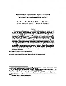
a b

c

Figure 1: An example of handling non-fixed input slew. Suppose that a buffer is to be inserted at position p and there are three immediate downstream buffers in a solution γ as shown in Figure 1. As the result upstream from p is not yet known, the input slew to the buffer can be in any slew bin. As such, in addition to C, W, S, each solution is augmented with new tuples L, U , which specify the lower bound and upper bound of the input slew to these immediate downstream buffers, respectively. In other words, the input slew is required to fall in [L, U ). Suppose that viewing at p, we have n(γ) immediate downstream buffers, each of which is associated with a lower bound Li and an upper bound Ui . Accordingly, there is an Si representing accumulated slew

3.1.3 Implementation Experiences We are to elaborate some implementation details in domination checking as well as domination elimination. In the algorithm, the solution set is stored using a linked list where elements are in no particular order. The straightforward lin-

310

corresponding to ψi (γ1 ). A bipartite graph is formed in this way since there are no links between nodes representing tuples in the same solution. For these two groups of vertices, the task is to answer whether there is a node-wise pairing (each from different groups) of cardinality n(γ1 ). We therefore reduce the problem to a maximum matching problem, which is to compute an edge set E  of maximum cardinality from E such that each vertex in V is incident to at most one edge of E  . Domination (on S, L, U ) follows if E  is of cardinality of n(γ1 ).

degradation viewing at each immediate downstream buffer. For example, in Figure 1, we have (S1 , L1 , U1 ) for the buffer inserted at a, (S2 , L2 , U2 ) for b, and (S3 , L3 , U3 ) for c. When a buffer is inserted at p, at most l new solutions are generated. They are with the same C, W, S values but with different L, U values. We say “at most” since whether a buffer with a certain input slew bin can be inserted at p needs to be validated. For a buffer b to be inserted with the input slew bin g, denote by [Sg , Sg ) the slew range of g. The buffer insertion is valid if for each immediate downstream buffer i (viewing at p, 1 ≤ i ≤ n(γ)) in γ, Li (γ) ≤

Sb,out

(p, g, C(γ))2

+ Si

(γ)2

≤ Ui (γ),

3.3 Continuous Slew Buffering What we have considered so far is the discrete slew buffering problem. It is expected that the total buffer area can be reduced if buffer positions are freely chosen in the routing tree. The following continuous slew buffering algorithm settles this problem. We begin with a simple case: Theorem 1: For a single buffer type, the optimal slew buffering can be computed in linear time. Proof (Sketch): In essence, the algorithm is only propagating a single candidate up to the source. To insert buffers along a single path, we place a buffer as far (i.e., upstream) as possible from the previously inserted buffer such that the slew constraint is still satisfied. When proceeding to a branching point, a buffer is also placed as upstream as possible while the slew constraint must be satisfied for both branches. It is easy to see that given n buffer positions and sinks, this greedy algorithm returns the optimal solution in O(n) time. 2 Note that the above greedy algorithm can work in either discrete or continuous case. We now generalize this idea to handle multiple buffer types. The major difficulty is, of course, every type of buffers can be inserted at a position. Within a single branch, after a new solution is generated (i.e., a buffer is inserted), it is placed into a priority queue, which is decreasingly ordered by the distance from the current buffer position to the root. The first element in the queue is then extracted as the next solution to be processed. The definition of domination (namely, γ1 dominates γ2 ) goes the same as before except that γ1 now needs to reside at a position no lower than γ2 . The above exponential algorithm is found to be inefficient by our experiment. As such, an approximation algorithm through adaptively selecting candidate buffers is proposed. All buffers with area less than a threshold (called filtered buffers) are first increasingly sorted according to their slew resistance. For a slew constraint α, the first c·(eα −1)·|B| buffers (note that all |B| buffers will be chosen when the value exceeds the number of filtered buffers) are selected to form the library for buffer insertion, where c is a constant and is experimentally determined to be 0.2. The idea behind this selection criterion reads as follows. Roughly speaking, for tight slew constraint, there will be many non-dominated solutions and thus our computation may only focus on a small number of buffers in order to reduce the size of the solution set. For loose slew constraint, a buffer will be inserted with a large gap from the previously inserted buffer and thus the solution set might not be very large. We can therefore choose more buffers (exponentially more in our case). Varying c, one can achieve different tradeoff between solution quality and runtime.

(4)

where Sb,out (p, g, C(γ)) is the output slew of the buffer b at p with g as its input slew bin and C(γ) as its downstream capacitance, and a lookup table is used to obtain its value. Upon validation, the buffer b is inserted to γ, the number of immediate downstream n(γ) is set to one, S1 (γ) is set to zero, and L1 (γ) = Sg and U1 (γ) = Sg . It is often valid for a buffer with numerous input slew bins to be inserted to the same solution γ. For efficiency reason, those new solutions are merged after buffer insertion. That is, after buffer insertion, two solutions γ1 and γ2 are merged to form γ  if C(γ1 ) = C(γ2 ), W (γ1 ) = W (γ2 ) and U1 (γ1 ) = L1 (γ2 ), where C, W, S of γ  remain unchanged while L1 (γ  ) = L1 (γ1 ) and U1 (γ  ) = U1 (γ2 ). Note that in branch merging, the parameter values (S, L, U ) of all immediate downstream buffers for a left-branch solution γ1 and a right-branch solution γ2 are stored together and n(γ  ) = n(γ1 ) + n(γ2 ). The definition of domination needs to be accordingly modified. For two solutions with the same number of immediate downstream buffers, domination is defined solely on C, W, Si , Li , Ui . In particular, the i-th buffer in γ1 and that in γ2 may refer to different immediate downstream buffers. This allows a fairly effective solution pruning procedure. Given two solutions γ1 and γ2 , we are to decide whether there is a pairing of immediate downstream buffers of γ1 and γ2 , respectively, such that Sπ1 (j) (γ1 ) ≤ Sπ2 (j) (γ2 ), Lπ1 (j) (γ1 ) ≤ Lπ2 (j) (γ2 ) and Uπ1 (j) (γ1 ) ≥ Uπ2 (j) (γ2 ) for each pair j where 1 ≤ j ≤ n(γ1 ) = n(γ2 ), and π(·) denotes the permutation of indices of immediate downstream buffers. If this is the case, together with C(γ1 ) ≤ C(γ2 ), W (γ1 ) ≤ W (γ2 ), we conclude that γ1 dominates γ2 . An example would be helpful to illustrate the above definition. Assume that γ1 , γ2 both have three immediate downstream buffers. Suppose that (Si , Li , Ui ) for γ1 are (3, 10, 60), (5, 30, 65), (3, 20, 50), and for γ2 are (5, 25, 35), (6, 50, 55), (10, 15, 35). γ1 dominates γ2 on (S, L, U ) since (3, 10, 60) dominates (10, 15, 35), (5, 30, 65) dominates (6, 50, 55), and (3, 20, 50) dominates (5, 25, 35). Given two solutions, we need to answer whether such pairing exists. The straightforward computation is inefficient since L, U may heavily overlap. As such, we reduce it to the maximum bipartite matching problem for an efficient solution. To check whether γ1 dominates γ2 , for each (Si (γ1 ), Li (γ1 ), Ui (γ1 )) in γ1 , a set of tuples, denoted by ψi (γ1 ), consisting of all (Sj (γ2 ), Lj (γ2 ), Uj (γ2 )) in γ2 is computed such that the former three-tuple dominates each of the latter three-tuples. A graph G = (V, E) is constructed as follows. Represent each three-tuple by a vertex. A vertex corresponding to the i-th tuple in γ1 links to the vertices

311

4.

• The number of buffers decreases and the area decreases for both algorithms as the slew constraint loosens. This makes sense since a looser constraint means that buffers can be spaced further apart. • SB is more efficient in area. For example, with a 1.0 ns slew constraint, the area savings is 5.9%. Note that the area savings increases with the slew constraint. It happens since VGL+S has fewer infeasible (i.e., violating slew constraints) solutions to throw away with a looser slew constraint, hence it is more likely to sacrifice area for delay. With a tight slew constraint, VGL+S has more limited choices since it must meet the slew constraint. Indeed, one can also see this by considering the number of candidates at the driver. • The slew buffering algorithm SB is much more efficient. Despite considering all 48 buffers in the library, it runs in just a few seconds on 1000 nets. Furthermore, it runs over 100 times faster than the timing buffering algorithm for a slew constraint α ≥ 1.1. The main reason for this fact is that there is a significantly smaller set of non-dominated solutions in slew buffering than in timing buffering. For example, when α = 1.0, we have only 12 solutions per net in the slew buffering, while the number is 310 in the slew constrained timing buffering. This is caused by the fact that slew gets to be reset to zero whenever a buffer is inserted, while delay has to be propagated up the entire tree. In practice, the runtime is virtually linear. • Comparing slack at driver, one sees that slew buffering achieves significant improvement in runtime with only slight scarification in slack. This suggests a new fast approximation for minimum cost timing driven buffering using our slew buffering algorithm.

DISCUSSION OF RELATED APPROACH

We refer to van Ginneken/Lillis’ algorithm as VGL and the discrete slew buffering algorithm with fixed input slew as SB. In order to make a meaningful comparison between them, we first modify VGL to handle a slew constraint, without modifying its delay objective function. The new slew constrained VGL is referred to as VGL+S. In this way, we can investigate the difference between simply handling the slew constraint to optimize delay versus handling the slew constraint to optimize cost. For this, the three-tuple (C, W, Q) is augmented to (C, W, Q, S), where Q denotes the required arrival time. Note that domination in timing buffering is defined on C, W, Q but not on S, while S is only responsible for eliminating infeasible solutions. In contrast, domination in slew buffering is defined on C, W, S but not on Q. Therefore, VGL+S algorithm may delete optimal solutions based on timing information while our new algorithm, with domination defined on C, W, S can find the minimum cost solution satisfying slew constraint. The experiments in the next section report the timing-driven buffering solution as the minimum cost solution at the driver, thereby slack at the driver plays no role. In this way, the impact of the actual change in optimization strategy for area instead of delay is considered.

5.

EXPERIMENTAL RESULTS

5.1 Experiment setup For convenience, all algorithms in comparison are listed below together with their abbreviations. • SB: discrete slew buffering algorithm with fixed input slew. • SB+NI: discrete slew buffering with non-fixed input slew. • C-SB: continuous slew buffering with fixed input slew. • VGL: van Ginneken/Lillis’ min-cost timing buffering algorithm. • VGL+S: slew constrained VGL.

It is worth mentioning that the range search tree pruning technique, when incorporated into SB, slows down the algorithm as indicated by our experiment. For example, when the slew constraint is 1.0, SB with range search tree returns the solution in 46.2 seconds compared to 6.1 seconds by the one without it. This fact is due to the considerable amount of inherent overhead in maintaining the balanced range search tree data structure.

All algorithms are implemented in C++ and are tested on a Pentium IV computer with a 3.2GHz CPU and 1G memory. Our test cases are extracted from an industrial ASIC chip, which consist of 1000 nets with more than 50 thousand nodes including sinks, branching nodes and buffer positions. Among them, 757 nets have ≤ 5 sinks and all the remaining nets have ≤ 20 sinks. The sink capacitances range from 2.5f F to 200f F . The wire resistance is 0.56Ω/µm and the wire capacitance is 0.48f F/µm. The buffer library consists of 48 buffers, in which 23 are non-inverting buffers and 25 are inverting buffers. Normalized buffer areas range from 5 to 34, slew resistances range from 0.18ns/pF to 29.3ns/pF , and input capacitances range from 2.1f F to 76.0f F .

5.3 Slew buffering with non-fixed input slew and continuous slew buffering Results of SB+NI and C-SB are summarized in Table 2. Area saving here refers to comparison to discrete slew buffering with fixed input slew, i.e., SB. We observe the following: • SB+NI can save up to 40% area over SB. In SB+NI, the number of input slew bins to each buffer is 21. For each slew bin, downstream capacitance is also discretized into 21 capacitance bins in the lookup table. With very tight slew constraint, SB+NI saves much more area over SB. It is the case since the actual input slew is significantly smaller than the pre-set upper bound. • SB+NI becomes slower with tighter slew constraint since the size of the solution set becomes much larger as more buffers are inserted. • In slew buffering, tighter constraint causes excessive buffer insertion. If the candidate buffer positions are not pre-set carefully in discrete slew buffering, we may often have to insert buffers in a very inefficient way.

5.2 Comparison with timing buffering We first compare SB with VGL+S, and results are summarized in Table 1. Here “area saving” refers to the percentage difference in area, “speed up” refers to the percentage difference in CPU time (seconds), and the slew constraint is given in nanoseconds. Note that in VGL+S, range search tree pruning is implemented as in [3]. We make the following observations:

312

Table 1: Comparison of discrete slew buffering and slew constrained timing buffering. #S@Dr: # nondominated solutions at driver.

Slew constraint (ns) 0.3 0.4 0.5 0.6 0.7 0.8 0.9 1.0 1.1 1.2 1.3 1.4 1.5 2.0 3.0

Optimal Discrete Slew Buffering (SB) Area # Buf Slack #S@Dr CPU (s) 49139 6545 8525 61 16.4 32738 6064 8585 53 15.3 23840 5124 8434 39 12.5 18512 4074 8643 26 9.3 15464 3529 8623 21 8.2 13231 3192 8504 16 7.4 11509 2933 8470 13 6.7 10231 2657 8436 12 6.1 9224 2362 8413 11 5.8 8376 2146 8392 10 5.9 7714 1972 8347 9 5.6 7143 1834 8296 9 5.7 6655 1695 8263 8 5.5 5189 1293 8016 6 4.8 3525 817 7694 5 4.9

Slew Constrained Area # Buf 49804 7273 34889 8713 25392 7618 19459 5237 16354 4511 14107 4270 12170 3724 10838 3337 9831 3023 8949 2754 8315 2569 7709 2404 7214 2255 5744 1850 4009 1304

Timing Buffering (VGL+S) Slack #S@Dr CPU (s) 8529 299 374.1 8813 269 394.2 8755 258 437.1 8776 271 475.3 8740 283 489.5 8678 289 522.3 8600 305 559.0 8550 310 586.3 8528 312 602.0 8487 320 621.4 8442 323 638.5 8406 328 654.0 8381 334 671.7 8217 342 737.5 8026 356 796.8

Ratio Area Saving Speed up 1.4% 22.8 6.6% 25.8 6.5% 35.0 5.1% 51.1 5.8% 59.7 6.6% 70.6 5.7% 83.4 5.9% 96.1 6.6% 103.8 6.8% 105.3 7.8% 114.0 7.9% 114.7 8.4% 122.1 10.7% 153.6 13.7% 162.6

Table 2: Results of slew buffering with non-fixed input slew and continuous slew buffering. Slew constraint (ns) 0.3 0.4 0.5 0.6 0.8 1.0 1.1 1.4 1.5 2.0 3.0

Discrete Area 35148 25018 19797 16528 12129 9629 8968 6947 6252 4813 3390

Slew Buffering With Non-Fixed Input Slew (SB+NI) # Buf CPU (s) Area Saving 7114 992.1 39.8% 5666 931.7 30.9% 4326 762.8 20.4% 3772 569.3 12.0% 3145 397.4 9.1% 2488 337.3 6.3% 2279 334.3 2.9% 1790 302.8 2.8% 1660 323.3 6.4% 1165 221.3 7.8% 775 194.3 3.9%

Continuous slew buffering (C-SB) significantly alleviates this problem and results in up to 26% improvement in buffer area. • C-SB runs very fast due to our adaptive procedure for buffer selection. If C-SB is carried out without buffer selection procedure, the algorithm becomes very slow. For example, we obtain a solution with buffer area 9291 in 1596.5 seconds for α = 1.0. Compared to C-SB with buffer selection, it is only 9330/9291 − 1 = 0.4% better in buffer area, however, it is 1596.5/21.7 > 70× slower.

6.

[3]

[4]

[5]

[6]

CONCLUSION

[7]

The slew buffering problem is intensively studied in this paper. Three new algorithms are proposed, namely, a slew buffering algorithm with the assumption of fixed input slew, a more sophisticated algorithm without this assumption, and a very efficient continuous slew buffering algorithm. Experimental results demonstrate that new algorithms run one to two orders of magnitude faster than the widely-used timing buffering algorithm and meanwhile they can obtain significant amount of area saving. Future work seeks to incorporate our results into a physical synthesis flow.

7.

[8]

[9]

[10]

REFERENCES

[11]

[1] P. Saxena and N. Menezes and P. Cocchini and D.A. Kirkpatrick, “Repeater scaling and its impact on CAD,” IEEE Transactions on Computer-Aided Design of Integrated Circuits and Systems, vol. 23, no. 4, pp. 451–463, 2004. [2] P.J. Osler, “Placement driven synthesis case studies on two sets of two chips: hierarchical and flat,” in Proceedings of the ACM

[12]

313

Continuous Slew Buffering (C-SB) Area # Buf CPU (s) Area Saving 38905 6616 2.7 26.3% 28745 4865 2.8 13.9% 21184 4284 9.4 12.5% 16930 4990 39.0 9.3% 11573 3063 27.7 14.3% 9330 2484 21.7 9.7% 8497 2222 19.1 8.6% 6806 1736 16.2 5.0% 6388 1645 14.8 4.2% 5089 1271 9.5 2.0% 3511 812 4.6 0.3%

International Symposium on Physical Design, pp. 190–197, 2004. J. Lillis and C.-K. Cheng and T.-T.Y. Lin, “Optimal wire sizing and buffer insertion for low power and a generalized delay model,” IEEE Journal of Solid State Circuits, vol. 31, no. 3, pp. 437–447, 1996. N. Menezes and C.-P. Chen, “Spec-based repeater insertion and wire sizing for on-chip interconnect,” in Proceedings of the IEEE International Conference on VLSI Design, pp. 476–483, 1999. C.J. Alpert and A. Devgan and S.T. Quay, “Buffer insertion for noise and delay optimization,” in Proceedings of the Design Automation Conference, pp. 362–367, 1998. ——, “Buffer insertion with accurate gate and interconnect delay computation,” in Proceedings of the Design Automation Conference, pp. 479–484, 1999. C.J. Alpert and A.B. Kahng and B. Liu and I. Mandoiu and A. Zelikovsky, “Minimum-buffered routing of non-critical nets for slew rate and reliability control,” in Proceedings of the International Conference on Computer Aided Design, pp. 408–415, 2001. C.J. Alpert and J. Hu and S.S. Sapatnekar and P.G. Villarrubia, “A practical methodology for early buffer and wire resource allocation,” in Proceedings of the Design Automation Conference, pp. 189–194, 2001. C.V. Kashyap and C.J. Alpert and F. Liu and A. Devgan, “Closed form expressions for extending step delay and slew metrics to ramp inputs,” in Proceedings of the International Symposium on Physical Design, pp. 24–31, 2003. H.B. Bakoglu, Circuits, Interconnects, and Packaging for VLSI. Addison-Wesley Publishing Company, 1990. N.H. Weste and K. Eshraghian, Principles of CMOS VLSI Design. Addison Wesley, 1993, pp. 221–223. L.P.P.P. van Ginneken, “Buffer placement in distributed RC-tree networks for minimal Elmore delay,” in Proceedings of the IEEE International Symposium on Circuits and Systems, pp. 865–868, 1990.