ter strings. The sorting algorithm blends Quicksort and radix sort; it is competitive
with the best known C sort codes. The searching algorithm blends tries and ...
Fast Algorithms for Sorting and Searching Strings Jon L. Bentley*
Abstract We present theoretical algorithms for sorting and searching multikey data, and derive from them practical C implementations for applications in which keys are character strings. The sorting algorithm blends Quicksort and radix sort; it is competitive with the best known C sort codes. The searching algorithm blends tries and binary search trees; it is faster than hashing and other commonly used search methods. The basic ideas behind the algorithms date back at least to the 1960s, but their practical utility has been overlooked. We also present extensions to more complex string problems, such as partial-match searching. 1. Introduction Section 2 briefly reviews Hoare’s [9] Quicksort and binary search trees. We emphasize a well-known isomorphism relating the two, and summarize other basic facts. The multikey algorithms and data structures are presented in Section 3. Multikey Quicksort orders a set of n vectors with k components each. Like regular Quicksort, it partitions its input into sets less than and greater than a given value; like radix sort, it moves on to the next field once the current input is known to be equal in the given field. A node in a ternary search tree represents a subset of vectors with a partitioning value and three pointers: one to lesser elements and one to greater elements (as in a binary search tree) and one to equal elements, which are then processed on later fields (as in tries). Many of the structures and analyses have appeared in previous work, but typically as complex theoretical constructions, far removed from practical applications. Our simple framework opens the door for later implementations. The algorithms are analyzed in Section 4. Many of the analyses are simple derivations of old results. Section 5 describes efficient C programs derived from the algorithms. The first program is a sorting algorithm __________________ * Bell Labs, Lucent Technologies, 700 Mountain Avenue, Murray Hill, NJ 07974;
[email protected]. # Princeton University, Princeton, NJ, 08544;
[email protected].
Robert Sedgewick#
that is competitive with the most efficient string sorting programs known. The second program is a symbol table implementation that is faster than hashing, which is commonly regarded as the fastest symbol table implementation. The symbol table implementation is much more space-efficient than multiway trees, and supports more advanced searches. In many application programs, sorts use a Quicksort implementation based on an abstract compare operation, and searches use hashing or binary search trees. These do not take advantage of the properties of string keys, which are widely used in practice. Our algorithms provide a natural and elegant way to adapt classical algorithms to this important class of applications. Section 6 turns to more difficult string-searching problems. Partial-match queries allow ‘‘don’t care’’ characters (the pattern ‘‘so.a’’, for instance, matches soda and sofa). The primary result in this section is a ternary search tree implementation of Rivest’s partial-match searching algorithm, and experiments on its performance. ‘‘Near neighbor’’ queries locate all words within a given Hamming distance of a query word (for instance, code is distance 2 from soda). We give a new algorithm for near neighbor searching in strings, present a simple C implementation, and describe experiments on its efficiency. Conclusions are offered in Section 7. 2. Background Quicksort is a textbook divide-and-conquer algorithm. To sort an array, choose a partitioning element, permute the elements such that lesser elements are on one side and greater elements are on the other, and then recursively sort the two subarrays. But what happens to elements equal to the partitioning value? Hoare’s partitioning method is binary: it places lesser elements on the left and greater elements on the right, but equal elements may appear on either side. Algorithm designers have long recognized the desirability and difficulty of a ternary partitioning method. Sedgewick [22] observes on page 244: ‘‘Ideally, we would like to get all [equal keys] into position in the file, with all
-2-
the keys with a smaller value to their left, and all the keys with a larger value to their right. Unfortunately, no efficient method for doing so has yet been devised....’’ Dijkstra [6] popularized this as ‘‘The Problem of the Dutch National Flag’’: we are to order a sequence of red, white and blue pebbles to appear in their order on Holland’s ensign. This corresponds to Quicksort partitioning when lesser elements are colored red, equal elements are white, and greater elements are blue. Dijkstra’s ternary algorithm requires linear time (it looks at each element exactly once), but code to implement it has a significantly larger constant factor than Hoare’s binary partitioning code. Wegner [27] describes more efficient ternary partitioning schemes. Bentley and McIlroy [2] present a ternary partition based on this counterintuitive loop invariant: =
< a
>
? b
c
= d
The main partitioning loop has two inner loops. The first inner loop moves up the index b: it scans over lesser elements, swaps equal elements to a, and halts on a greater element. The second inner loop moves down the index c correspondingly: it scans over greater elements, swaps equal elements to d, and halts on a lesser element. The main loop then swaps the elements pointed to by b and c, increments b and decrements c, and continues until b and c cross. (Wegner proposed the same invariant, but maintained it with more complex code.) Afterwards, the equal elements on the edges are swapped to the middle of the array, without any extraneous comparisons. This code partitions an n-element array using n − 1 comparisons. Quicksort has been extensively analyzed by authors including Hoare [9], van Emden [26], Knuth [11], and Sedgewick [23]. Most detailed analyses involve the harmonic numbers H n = Σ 1≤i≤n 1/ i. Theorem 1. [Hoare] A Quicksort that partitions around a single randomly selected element sorts n distinct items in 2nH n + O(n) ∼ ∼ 1. 386n lg n expected comparisons. A common variant of Quicksort partitions around the median of a random sample. Theorem 2. [van Emden] A Quicksort that partitions around the median of 2t + 1 randomly selected elements sorts n distinct items in 2nH n / (H 2t + 2 − H t + 1 ) + O(n) expected comparisons. By increasing t, we can push the expected number of comparisons close to n lg n + O(n). The theorems so far deal only with the expected performance. To guarantee worst-case performance, we partition
31
41
59
26
53
26
31
41
59
53
41
59
53
53
59
26
53
31 26
41 59 53
Figure 1. Quicksort and a binary search tree around the true median, which can be computed in cn comparisons. (Schoenhage, Paterson and Pippenger [20] give a worst-case algorithm that establishes the constant c = 3; Floyd and Rivest [8] give an expected-time algorithm with c = 3/2.) Theorem 3. A Quicksort that partitions around a median computed in cn comparisons sorts n elements in cn lg n + O(n) comparisons. The proof observes that the recursion tree has about lg n levels and does at most cn comparisons on each level. The Quicksort algorithm is closely related to the data structure of binary search trees (for more on the data structure, see Knuth [11]). Figure 1 shows the operation of both on the input sequence ‘‘31 41 59 26 53’’. The tree on the right is the standard binary search tree formed by inserting the elements in input order. The recursion tree on the left shows an ‘‘ideal partitioning’’ Quicksort: it partitions around the first element in its subarray and leaves elements in both subarrays in the same relative order. At the first level, the algorithm partitions around the value 31, and produces the left subarray ‘‘26’’ and the right subarray ‘‘41 59 53’’, both of which are then sorted recursively. Figure 1 illustrates a fundamental isomorphism between Quicksort and binary search trees. The (unboxed) partitioning values on the left correspond precisely to the internal nodes on the right in both horizontal and vertical placement. The internal path length of the search tree is the total number of comparisons made by both structures. Not only are the totals equal, but each structure makes the same set of comparisons. The expected cost of a successful search is, by definition, the internal path length divided by n. We combine that with Theorem 1 to yield Theorem 4. [Hibbard] The average cost of a successful search in a binary search tree built by inserting elements in random order is 2H n + O( 1 ) ∼ ∼ 1. 386 lg n comparisons. An analogous theorem corresponds to Theorem 2: we can reduce the search cost by choosing the root of a subtree to be the median of 2t + 1 elements in the subtree. By analogy to Theorem 3, a perfectly balanced subtree decreases the search time to about lg n.
-3-
3. The Algorithms Just as Quicksort is isomorphic to binary search trees, so (most-significant-digit) radix sort is isomorphic to digital search tries (see Knuth [11]). These isomorphisms are described in this table: ____________________________________ ____________________________________ Algorithm Data Structure ____________________________________ Quicksort Binary Search Trees Multikey Quicksort Ternary Search Trees MSD Radix Sort Tries ____________________________________
This section introduces the algorithm and data structure in the middle row of the table. Like radix sort and tries, the structures examine their input field-by-field, from most significant to least significant. But like Quicksort and binary search trees, the structures are based on field-wise comparisons, and do not use array indexing. We will phrase the problems in terms of a set of n vectors, each of which has k components. The primitive operation is to perform a ternary comparison between two components. Munro and Raman [18] describe an algorithm for sorting vector sets in-place, and their references describe previous work in the area. Hoare [9] sketches a Quicksort modification due to P. Shackleton in a section on ‘‘Multi-word Keys’’: ‘‘When it is known that a segment comprises all the items, and only those items, which have key values identical to a given value over the first n words, in partitioning this segment, comparison is made of the (n + 1 )th word of the keys.’’ Hoare gives an awkward implementation of this elegant idea; Knuth [11] gives details on Shackleton’s scheme in Solution 5.2.2.30. A ternary partitioning algorithm provides an elegant implementation of Hoare’s multikey Quicksort. This recursive pseudocode sorts the sequence s of length n that is known to be identical in components 1..d − 1; it is originally called as sort(s, n, 1). sort(s, n, d) if n ≤ 1 or d > k return; choose a partitioning value v; partition s around value v on component d to form sequences s < , s = , s > of sizes n < , n = , n > ; sort(s < , n < , d); sort(s = , n = , d + 1); sort(s > , n > , d); The partitioning value can be chosen in many ways, from computing the true median of the specified component to choosing a random value in the component. Ternary search trees are isomorphic to this algorithm. Each node in the tree contains a split value and pointers to low and high (or left and right) children; these fields per-
i b a
s
e
s
h y
e
n
o t
n f
t r
o
t as at be by he in is it of on or to
Figure 2. A ternary search tree for 12 two-letter words form the same roles as the corresponding fields in binary search trees. Each node also contains a pointer to an equal child that represents the set of vectors with values equal to the split value. If a given node splits on dimension d, its low and high children also split on d, while its equal child splits on d + 1. As with binary search trees, ternary trees may be perfectly balanced, constructed by inserting elements in random order, or partially balanced by a variety of schemes. In Section 6.2.2, Knuth [11] builds an optimal binary search tree to represent the 31 most common words in English; twelve of those words have two letters. Figure 2 shows the perfectly balanced ternary search tree that results from viewing those words as a set of n = 12 vectors of k = 2 components. The low and high pointers are shown as solid lines, while equal pointers are shown as dashed lines. The input word is shown beneath each terminal node. This tree was constructed by partitioning around the true median of each subset. A search for the word ‘‘is’’ starts at the root, proceeds down the equal child to the node with value ‘‘s’’, and stops there after two comparisons. A search for ‘‘ax’’ makes three comparisons to the first letter (‘‘a’’) and two comparisons to the second letter (‘‘x’’) before reporting that the word is not in the tree. This idea dates back at least as far as 1964; see, for example, Clampett [5]. Prior authors had proposed representing the children of a trie node by an array or by a linked list; Clampett represents the set of children with a binary search tree; his structure can be viewed as a ternary search tree. Mehlhorn [17] proposes a weight-balanced ternary search tree that searches, inserts and deletes elements in a set of n strings of length k in O( log n + k) time; a similar structure is described in Section III.6.3 of Mehlhorn’s text [16]. Bentley and Saxe [4] propose a perfectly balanced ternary search tree structure. The value of each node is the median of the set of elements in the relevant dimension; the tree in Figure 1 was constructed by this criterion. Bentley and Saxe present the structure as a solution to a
-4-
problem in computational geometry; they derive it using the geometric design paradigm of multidimensional divide-and-conquer. Ternary search trees may be built in a variety of ways, such as by inserting elements in input order or by building a perfectly balanced tree for a completely specified set. Vaishnavi [25] and Sleator and Tarjan [24] present schemes for balancing ternary search trees. 4. Analysis We will start by analyzing ternary search trees, and then apply those results to multikey Quicksort. Our first theorem is due to Bentley and Saxe [4]. Theorem 5. [Bentley and Saxe] A search in a perfectly balanced ternary search tree representing n k-vectors requires at most lg n + k scalar comparisons, and this is optimal. Proof Sketch. For the upper bound, we start with n active vectors and k active dimensions; each comparison halves the active vectors or decrements the active dimensions. For the lower bound, consider a vector set in which all elements are equal in the first k − 1 dimensions and distinct in the k th dimension. Similar search times for the suffix tree data structure are reported by Manber and Myers [14]. We will next consider the multikey Quicksort that always partitions around the median element of the subset. This theorem corresponds to Theorem 3. Theorem 6. If multikey Quicksort partitions around a median computed in cn comparisons, it sorts n kvectors in at most cn( lg n + k) scalar comparisons. Proof. Because the recursion tree is perfectly balanced, no node is further than lg n + k from the root by Theorem 5. Each level of the tree contains at most n elements, so by the linearity of the median algorithm, at most cn scalar comparisons are performed at each level. Multiplication yields the desired result. A multikey Quicksort that partitions around a randomly selected element requires at most n( 2H n + k + O( 1 ) ) comparisons, by analogy with Theorem 1. We can further decrease that number by partitioning around a sample median. Theorem 7. A multikey Quicksort that partitions around the median of 2t + 1 randomly selected elements sorts n k-vectors in at most 2nH n / (H 2t + 2 − H t + 1 ) + O(kn) expected scalar comparisons. Proof Sketch. Combine Theorem 2 with the observation that equal elements strictly decrease the number of comparisons. The additive cost of O(kn) accounts for inspecting all k keys.
By increasing the sample size t, one can reduce the time to near n lg n + O(kn). (Munro and Raman [18] describe an in-place vector sort with that running time.) We will now turn from sorting to analogous results about building ternary search trees. We can build a tree from scratch in the same time bounds described above: adding ‘‘bookkeeping’’ functions (but no additional primitive operations) augments a sort to construct a tree as well. Given sorted input, the tree can be built in O(kn) comparisons. Theorem 6 describes the worst-case cost of searching in a totally balanced tree. The expected number of comparisons used by a successful search in a randomly built tree is 2H n + k + O( 1 ); partitioning around a sample median tightens that result. Theorem 8. The expected number of comparisons in a successful search in a ternary search tree built by partitioning around the median of 2t + 1 randomly selected elements is 2H n / (H 2t + 2 − H t + 1 ) + k + O( 1 ). Proof Sketch. Use Theorem 7 and the isomorphism between trees and sort algorithms. 5. String Programs The ideas underlying multikey Quicksort and ternary search trees are simple and old, and they yield theoretically efficient algorithms. Their utility for the case when keys are strings has gone virtually unnoticed, which is unfortunate because string keys are common in practical applications. In this section we show how the idea of ternary recursive decomposition, applied character-by-character on strings, leads to elegant and efficient C programs for sorting and searching strings. This is the primary practical contribution of this paper. We assume that the reader is familiar with the C programming language described by Kernighan and Ritchie [10]. C represents characters as small integers, which can be easily compared. Strings are represented as vectors of characters. The structures and theorems that we have seen so far apply immediately to sets of strings of a fixed length. Standard C programs, though, use variable-length strings that are terminated by a null character (the integer zero). We will now use multikey Quicksort in a C function to sort strings.* The primary sort function has this declaration: void ssort1main(char *x[], int n)
It is passed the array x of n pointers to character strings; its job is to permute the pointers so the strings occur in lex__________________ * The program (and other related content) is available http://www.cs.princeton.edu/˜rs/strings.
at
-5-
icographically nondecreasing order. We will employ an auxiliary function that is passed both of those arguments, and an additional integer depth to tell which characters are to be compared. The algorithm terminates either when the vector contains at most one string or when the current depth ‘‘runs off the end’’ of the strings. The sort function uses these supporting macros. #define swap(a, b) { char *t=x[a]; \ x[a]=x[b]; x[b]=t; } #define i2c(i) x[i][depth]
The swap macro exchanges two pointers in the array and the i2c macro (for ‘‘integer to character’’) accesses character depth of string x[i]. A vector swap function moves sequences of equal elements from their temporary positions at the ends of the array back to their proper place in the middle. void vecswap(int i, int j, int n, char *x[]) { while (n-- > 0) { swap(i, j); i++; j++; } }
The complete sorting algorithm is in Program 1; it is similar to the code of Bentley and McIlroy [2]. The function is originally called by void ssort1main(char *x[], int n) { ssort1(x, n, 0); }
After partitioning, we recursively sort the lesser and greater segments, and sort the equal segment if the corresponding character is not zero. We can tune the performance of Program 1 using standard techniques such as those described by Sedgewick [21]. Algorithmic speedups include sorting small subarrays with insertion sort and partitioning around the median of three elements (and on larger arrays, the median of three medians of three) to exploit Theorem 7. Standard C coding techniques include replacing array indices with pointers. This table gives the number of seconds required to sort a /usr/dict/words file that contains 72,275 words and 696,436 characters. _____________________________________________________ ___________________________________________________ Machine MHz System Simple Tuned Radix ____________________________________________________ MIPS R4400 150 .85 .79 .44 .40 MIPS R4000 100 1.32 1.30 .68 .62 Pentium 90 1.74 .98 .69 .50 486DX 33 8.20 4.15 2.41 1.74 ____________________________________________________
The third column reports the time of the system qsort function, and the fourth column reports the time of Program 1. Our simple code is always as fast as the (generalpurpose but presumably highly tuned) system function, and sometimes much faster. The fifth column reports the time
void ssort1(char *x[], int n, int depth) { int a, b, c, d, r, v; if (n lokid; else if (*s == p->splitchar) if (*s++ == 0) return 1; p = p->eqkid; } else p = p->hikid; } return 0; }
number of branches taken over all possible successful searches in the tree. The results are presented in this table:
{
Program 2. Search a ternary search tree Tptr insert1(Tptr p, char *s) { if (p == 0) { p = (Tptr) malloc(sizeof(Tnode)); p->splitchar = *s; p->lokid = p->eqkid = p->hikid = 0; } if (*s < p->splitchar) p->lokid = insert1(p->lokid, s); else if (*s == p->splitchar) { if (*s != 0) p->eqkid = insert1(p->eqkid, ++s); } else p->hikid = insert1(p->hikid, s); return p; }
Program 3. Insert into a ternary search tree typedef struct tnode *Tptr; typedef struct tnode { char splitchar; Tptr lokid, eqkid, hikid; } Tnode;
The value stored at the node is splitchar, and the three pointers represent the three children. The root of the tree is declared to be Tptr root;. Program 2 returns 1 if string s is in the tree and 0 otherwise. It starts at the root, and moves down the tree. The lokid and hikid branches are obvious. Before it takes a eqkid branch, it returns 1 if the current character is the end-of-string character 0. After the loop, we know that we ran off the tree while still looking for the string, so we return 0. Program 3 inserts a new string into the tree (and does nothing if it is already present). We insert the string s with the code root = insert(root, s). The first if statement detects running off the end of the tree; it then makes a new node, initializes it, and falls through to the standard case. Subsequent code takes the appropriate branch, but branches to eqkid only if characters remain in the string. We tested the search performance on the same dictionary used for testing sorting. We inserted each of the 72,275 words into the tree, and then measured the average
__________________________________________________ ________________________________________________ Input Branches Nodes Lo Order Eq Hi Total _________________________________________________ Balanced 285,807 4.39 9.64 3.91 17.94 Tournament 285,807 5.04 9.64 4.62 19.30 285,807 5.26 Random 9.64 5.68 20.58 Dictionary 285,807 0.06 9.64 31.66 41.36 Sorted 285,807 0 9.64 57.72 67.36 9.64 0 47.04 _Reversed ________________________________________________ 285,807 37.40
The rows describe six different methods of inserting the strings into the tree. The first column immediately suggests this theorem. Theorem 11. The number of nodes in a ternary search tree is constant for a given input set, independent of the order in which the nodes are inserted. Proof. There is a unique node in the tree corresponding to each unique string prefix in the set. The relative positions of the nodes within the tree can change as a function of insertion order, but the number of nodes is invariant. Notice that a standard search trie (without node compaction) would have exactly the same number of nodes. In this data set, the number of nodes is only about 41 percent of the number of characters. The average word length (including delimiter characters) is 696 , 436/72 , 275 ∼ ∼ 9.64 characters. The average number of equal branches in a successful search is precisely 9.64, because each input character is compared to an equal element once. The balanced tree always chooses the root of a subtree to be the median element in that collection. In that tree, the number of surplus (less and greater) comparisons is only 8.30 (about half the worst-case bound of 16 of Theorem 5), so the total number of comparisons is just 17.94. To build the tournament tree, we first sort the input set. The recursive build function inserts the middle string of its subarray, and then recursively builds the left and right subarrays. This tree uses about eight percent more comparisons than the balanced tree. The randomly built tree uses just fifteen percent more comparisons. The fourth line of the table describes inserting the words in dictionary order (which isn’t quite sorted due to capital letters and special characters). The final two lines describe inserting the words in sorted order and in reverse sorted order. These inputs slow down the search by a factor of at most four; in a binary search tree, they slow down the search by a factor of over 2000. Ternary search trees appear to be quite robust.
-7-
We conducted simple experiments to see how ternary search trees compare to other symbol table structures described by Knuth [11]. We first measured binary search, which can be viewed as an implementation of perfectly balanced binary search trees. For the same input set, binary search uses 15.19 string comparisons and inspects 51.74 characters, on the average (the average string comparison inspects 3.41 characters). On all computers we tested, a highly tuned binary search took about twice the time of Program 2 (on a tournament tree). The typical implementation of symbol tables is hashing. To represent n strings, we will use a chained hash table of size tabsize = n. The hash function is from Section 6.6 of Kernighan and Ritchie [10]; it is reasonably efficient and produces good spread. int hashfunc(char *s) { unsigned n = 0; for ( ; *s; s++) n = 31 * n + *s; return n % tabsize; }
Here is the body of the search function: for (p = tab[hashfunc(s)]; p; p = p->next) if (strcmp(s, p->str) == 0) return 1; return 0;
For fair timing, we replaced the string comparison function strcmp with inline code (so this hash and tree search functions used the same coding style). On the same dictionary, the average successful hash search requires 1.50 string comparisons (calls to the strcmp function) and 10.17 character comparisons (a successful search requires one comparison to the stored string, and half a comparison to the string in front of it, which almost always ends on the first character). In addition, every search must compute the hash function, which usually inspects every character of the input string. These simple experiments show that ternary search trees are competitive with the best known symbol table structures. There are, however, many ways to improve ternary search trees. The search function in Program 2 is reasonably efficient; tuning techniques such as saving the difference between compared elements, reordering tests, and using registers squeeze out at most an additional ten percent. This table compares the time of the resulting program with a similarly tuned hash function: _____________________________________________ _____________________________________________ Successful Unsuccessful Machine MHz TST Hash TST Hash _____________________________________________ MIPS R4400 150 .44 .43 .27 .39 MIPS R4000 100 .66 .61 .42 .54 Pentium 90 .58 .65 .38 .50 486DX 33 2.21 2.16 1.45 1.55 _____________________________________________
The times are the number of seconds required to perform a search for every word in the dictionary. For successful searches, the two structures have comparable search times. We generated unsuccessful searches by incrementing the first character of the word (so bat is transformed to the word cat, and cat is transformed to the nonword dat). Ternary search trees are faster than hashing for this simple model and others. Models for unsuccessful search are application-dependent, but ternary search trees are likely to be faster than hashing for unsuccessful search in applications because they can discover mismatches after examining only a few characters, while hashing always processes the entire key. For the long keys typical of some applications, the advantage is even more important than for the simple dictionary considered here. On the DIMACS library call number data sets, for instance, our program took less than one-fifth the time of hashing. The insert function in Program 3 has much room for improvement. Tournament tree insertion (inserting the median element first, and then recursively inserting the lesser and greater elements) provides a reasonable tradeoff between build and search times. Replacing the call to the memory allocation function malloc with a buffer of available nodes almost eliminates the time spent in memory allocation. Other common techniques also reduced the run time: transforming recursion to iteration, keeping a pointer to a pointer, reordering tests, saving a difference in a comparison, and splitting the single loop into two loops. The combination of these techniques sped up Program 3 by a factor of two on all machines we have been considering, and much more in environments with a slow malloc. In our experiments, the cost of inserting all the words in the dictionary is never more than about fifty percent greater than searching for all words with Program 2. The efficient insertion routine requires 35 lines of C; it can be found on our Web page cited earlier. The main drawback of ternary search trees compared to hashing is their space requirements. Our ternary search tree uses 285,807 16-byte nodes for a total of 4.573 megabytes. Hashing uses a hash table of 72,275 pointers, 72,275 8-byte nodes, and 696,436 bytes of text, for 1.564 megabytes. An alternative representation of ternary search trees is more space-efficient: when a subtree contains a single string, we store a pointer to the string itself (and each node stores three bits telling whether its children point to nodes or strings). This leads to slower and more complex code, but it reduces the number of tree nodes from 285,807 to 94,952, which is close to the space used by hashing. Ternary search trees can efficiently answer many kinds of queries that require linear time in a hash table. As in most ordered search trees, logarithmic-time searches can
-8-
find the predecessor or successor of a given element or count the number of strings in a range. Similarly, a tree traversal reports all strings in sorted order in linear time. We will see more advanced searches in the next section. In summary, ternary search trees seem to combine the best of two worlds: the low overhead of binary search trees (in terms of space and run time) and the character-based efficiency of search tries. The primary challenge in using tries in practice is to avoid using excessive memory for trie nodes that are nearly empty. Ternary search trees may be thought of as a trie implementation that gracefully adapts to handle this case, at the cost of slightly more work for full nodes. Ternary search trees are also easy to implement; compare our code, for instance, to Knuth’s implementation of ‘‘hash tries’’ [3] . Ternary search trees have been used for over a year to represent English dictionaries in a commercial Optical Character Recognition (OCR) system built at Bell Labs. The trees were faster than hashing for the task, and they gracefully handle the 34,000-character set of the Unicode Standard. The designers have also experimented with using partial-match searching for word lookup: replace letters with low probability of recognition with the ‘‘don’t care’’ character. 6. Advanced String Search Algorithms We will turn next to two search algorithms that have not been analyzed theoretically. We begin with the venerable problem of ‘‘partial-match’’ searching: a query string may contain both regular letters and the ‘‘don’t care’’ character ‘‘.’’. Searching the dictionary for the pattern ‘‘.o.o.o’’ matches the single word rococo, while the pattern ‘‘.a.a.a’’ matches many words, including banana, casaba, and pajama. This problem has been studied by many researchers, including Appel and Jacobson [1] and Manber and BaezaYates [13]. Rivest [19] presents an algorithm for partialmatch searching in tries: take the single given branch if a letter is specified, for a don’t-care character, recursively search all branches. Program 4 implements Rivest’s method in ternary search trees; it is called, for instance, by srchtop = 0; pmsearch(root, ".a.a.a");
Program 4 has five if statements. The first returns when the search runs off the tree. The second and fifth if statements are symmetric; they recursively search the lokid (or hikid) when the search character is the don’t care ‘‘.’’ or when the search string is less (or greater) than the splitchar. The third if statement recursively searches the eqkid if both the splitchar and current character in the query string are non-null. The fourth if
char *srcharr[100000]; int srchtop; void pmsearch(Tptr p, char *s) { if (!p) return; nodecnt++; if (*s == ’.’ || *s < p->splitchar) pmsearch(p->lokid, s); if (*s == ’.’ || *s == p->splitchar) if (p->splitchar && *s) pmsearch(p->eqkid, s+1); if (*s == 0 && p->splitchar == 0) srcharr[srchtop++] = (char *) p->eqkid; if (*s == ’.’ || *s > p->splitchar) pmsearch(p->hikid, s); }
Program 4. Partial match search statement detects a match to the query and adds the pointer to the complete word (stored in eqkid because the storestring flag in Program 4 is nonzero) to the output search array srcharr. Rivest states that partial-match search in a trie requires ‘‘time about O(n (k − s)/ k ) to respond to a query word with s letters specified, given a file of n k-letter words’’. Ternary search trees can be viewed as an implementation of his tries (with binary trees implementing multiway branching), so we expected his results to apply immediately to our program. Our experiments, however, led to a surprise: unspecified positions at the front of the query word are dramatically more costly than unspecified characters at the end of the word. For the same dictionary we have already seen, Table 1 presents the queries, the number of matches, and the number of nodes visited during the search in both a balanced tree and a random tree. To study this phenomenon, we have conducted experiments on both the dictionary and on random data (which closely models the dictionary). The page limit of these proceedings does not allow us to describe those experiments, which confirm the anecdotes in the above table. The key insight is that the top levels of a trie representing the dictionary have very high branching factor; a starting don’t-care character usually implies 52 recursive searches. Near the end of the word, though, the branching factor tends to be small; a don’t-care character at the end of the word frequently gives just a single recursive search. For this very reason, Rivest suggests that binary tries should ‘‘branch on the first bit of the representation of each character ... before branching on the second bit of each’’. Flajolet and Puech [7] analyzed this phenomenon in detail for bit tries; their methods can be extended to provide a detailed explanation of search costs as a function of unspecified query positions.
-9___________________________________________ _____________________________________________ ___________________ Nodes Pattern Matches Random Balanced ____________________________________________ television 1 18 24 tele...... 17 261 265 t.l.v.s..n 1 153 164 37,178 ....vision 1 36,484 banana 1 15 17 ban... 15 166 166 .a.a.a 19 2829 2746 ...ana 8 14,056 13,756 abracadabra 1 21 17 .br.c.d.br. 1 244 266 a..a.a.a..a 1 1127 1104 xy....... 3 67 66 157,449 .......xy 3 156,145 45 1 _. ___________________________________________ 285,807 285,807
Table 1. Partial match search performance We turn finally to the problem of ‘‘near-neighbor searching’’ in a set of strings: we are to find all words in the dictionary that are within a given Hamming distance of a query word. For instance, a search for all words within distance two of soda finds code, coma and 117 other words. Program 5 performs a near neighbor search in a ternary search tree. Its three arguments are a tree node, a string, and a distance. The first if statement returns if the node is null or the distance is negative. The second and fourth if statements are symmetric: they search the appropriate child if the distance is positive or if the query character is on the appropriate side of splitchar. The third if statement either checks for a match or recursively searches the middle child. We have conducted extensive experiments on the efficiency of Program 5; space limits us to sketching just one experiment. This table describes its performance on two similar data sets: void nearsearch(Tptr p, char *s, int d) { if (!p || d < 0) return; nodecnt++; if (d > 0 || *s < p->splitchar) nearsearch(p->lokid, s, d); if (p->splitchar == 0) { if ((int) strlen(s) eqkid; } else nearsearch(p->eqkid, *s ? s+1:s, (*s==p->splitchar) ? d:d-1); if (d > 0 || *s > p->splitchar) nearsearch(p->hikid, s, d); }
Program 5. Near neighbor search
____________________________________________________ ______________________________________________________ Dictionary Random D Min Min Mean Max Mean Max _____________________________________________________ 0 9 17.0 22 9 17.1 22 1 228 403.5 558 188 239.5 279 2 1374 2455.5 3352 1690 1958.7 2155 3 6116 8553.7 10829 7991 8751.3 9255 18268.3 21603 20751 21537.1 21998 _4____________________________________________________ 15389
The first line shows the costs for performing searches of distance 0 from each word in the data set. The ‘‘Dictionary’’ data represented the 10,451 8-letter words in the dictionary in a tree of 55,870 nodes. A distance-0 search was performed for every word in the dictionary. The minimum-cost search visited 9 nodes (to find latticed) and the maximum-cost search visited 22 nodes (to find woodnote), while the mean search cost was 17.0. The ‘‘Random’’ data represented 10,000 8-letter words randomly generated from a 10-symbol alphabet in a tree of 56,886 nodes. Subsequent lines in the table describe search distances 1 through 4. This simple experiment shows that searching for near neighbors is relatively efficient, searching for distant neighbors grows more expensive, and that a simple probabilistic model accurately predicts the time on the real data. 7. Conclusions Sections 3 and 4 used old techniques in a uniform presentation and analysis of multikey Quicksort and ternary search trees. This uniform framework led to the code in later sections. Multikey Quicksort leads directly to Program 1 and its tuned variant, which is competitive with the best known algorithms for sorting strings. This does not, however, exhaust the application of the underlying algorithm. We believe that multikey Quicksort might also be practical in multifield system sorts, such as that described by Linderman [12]. One might also use the algorithm to sort integers, for instance, by comparing them byte-by-byte. Section 5 shows that ternary search trees provide an efficient implementation of string symbol tables, and Section 6 shows that the structures can quickly answer more advanced queries. Ternary search trees are particularly appropriate when search keys are long strings, and they have already been incorporated into a commercial system. Advanced searching algorithms based on ternary search trees are likely to be useful in practical applications, and they present a number of interesting problems in the analysis of algorithms. Acknowledgments We are grateful for the helpful comments of Raffaele Giancarlo, Doug McIlroy, Ian Munro and Chris Van Wyk.
- 10 -
References 1. Appel, A.W. and Jacobson, G.J. The World’s Fastest Scrabble Program. Communications of the ACM 31, 5 (May 1988), 572-578. 2. Bentley, J.L. and McIlroy, M.D. Engineering A Sort Function. Software-Practice and Experience 23, 1 (1993), 1249-1265. 3. Bentley, J.L., McIlroy, M.D., and Knuth, D.E. Programming Pearls: A Literate Program. Communications of the ACM 29, 6 (June 1986), 471-483. 4. Bentley, J.L. and Saxe, J.B. Algorithms on Vector Sets. SIGACT News 11, 9 (Fall 1979), 36-39. 5. Clampett, H.A. Jr. Randomized Binary Searching with Tree Structures. Communications of the ACM 7, 3 (March 1964), 163-165. 6. Dijkstra, E.W. A Discipline of Programming. Prentice-Hall, Englewood Cliffs, NJ, 1976. 7. Flajolet, P. and Puech, C. Partial Match Retrieval of Multidimensional Data. Journal of the ACM 33, 2 (April 1986), 371-407. 8. Floyd, R.W. and Rivest, R.L. Expected Time Bounds for Selection. Communications of the ACM 18, 3 (March 1975), 165-172. 9. Hoare, C.A.R. Quicksort. Computer Journal 5, 1 (April 1962), 10-15. 10. Kernighan, B.W. and Ritchie, D.M. The C Programming Language, Second Edition. Prentice-Hall, Englewood Cliffs, NJ, 1988. 11. Knuth, D.E. The Art of Computer Programming, volume 3: Sorting and Searching. Addison-Wesley, Reading, MA, 1975. 12. Linderman, J.P. Theory and Practice in the Construction of a Working Sort Routine. Bell System Technical Journal 63, 8 (October 1984), 1827-1843. 13. Manber, U. and Baeza-Yates, R. An Algorithm for String Matching with a Sequence of Don’t Cares. Information Processing Letters 37, 3 (February 1991), 133-136. 14. Manber, U. and Myers, G. Suffix Arrays: A New
Method for On-Line String Searches. SIAM Journal on Computing 22 (1993), 935-948. 15. McIlroy, P.M., Bostic, K., and McIlroy, M.D. Engineering Radix Sort. Computing Systems 6, 1 (1993), 5-27. 16. Mehlhorn, K. Data Structures and Algorithms 1: Sorting and Searching. Springer-Verlag, Berlin, 1984. 17. Mehlhorn, K. Dynamic Binary Search. SIAM Journal on Computing 8, 2 (May 1979), 175-198. 18. Munro, J.I. and Raman, V. Sorting Multisets and Vectors In-Place. Proceedings of the Second Workshop on Algorithms and Data Structures, Springer Verlag Lecture Notes in Computer Science 519 (1991), 473-480. 19. Rivest, R.L. Partial-Match Retrieval Algorithms. SIAM Journal on Computing 5, 1 (1976), 19-50. 20. Schoenhage, A.M., Paterson, M., and Pippenger, N. Finding the Median. Journal of Computer and Systems Sciences 13 (1976), 184-199. 21. Sedgewick, R. Implementing Quicksort Programs. Communications of the ACM 21, 10 (October 1978), 847-857. 22. Sedgewick, R. Quicksort With Equal Keys. SIAM J. Comp 6, 2 (June 1977), 240-267. 23. Sedgewick, R. The Analysis of Quicksort Programs. Acta Informatica 7 (1977), 327-355. 24. Sleator, D.D. and Tarjan, R.E. Self-Adjusting Binary Search Trees. Journal of the ACM 32, 3 (July 1985), 652-686. 25. Vaishnavi, V.K. Multidimensional Height-Balanced Trees. IEEE Transactions on Computers C-33, 4 (April 1984), 334-343. 26. van Emden, M.H. Increasing the Efficiency of Quicksort. Communications of the ACM 13, 9 (September 1970), 563-567. 27. Wegner, L.M. Quicksort for Equal Keys. IEEE Transactions on Computers C-34, 4 (April 1985), 362-367.