to create a narrow band of the image points lying within a given distance to .... Sethian, J.A.: Level Set Methods and Fast Marching Methods: Evolving Interfaces.
Fast and Accurate Redistancing for Level Set Methods. Karl Krissian, Carl-Fredrik Westin Harvard Medical School Brigham and Women’s Hospital Dep of Radiology Thorn 323 Boston, MA 02115 USA {karl,westin}@bwh.harvard.edu ??
Introduction Although the Level Set Method [4] has only recently been introduced as an image processing tool, it has already proved useful in delineating contours and in segmenting objects. However, since this method represents contours with images, processing time may increase considerably. To offset this problem, it is common to create a narrow band of the image points lying within a given distance to the contour, and then process the contour evolution inside this narrow band. The use of the narrow band and numerical considerations require computing the distance to the evolving contour every few iterations. Several techniques have been proposed for computing this distance [2, 5]. In [1], the authors identify the problem of preserving the exact position of the interface and propose to solve a new Partial Differential Equation for this purpose. In [5], a nlog(n) algorithm is proposed to compute the distance by propagation until a given distance to the contour is reached. In this paper, we present two improvements: 1) We estimate the Euclidean distance to the interpolated surface for all voxels that are neighbors to the surface; and 2) We apply a fast approximation of the Distance Transform only in the narrow band, which, in turn, reduces the complexity of nlog(n) to n, where n is the size of the narrow band.
Sub-Voxel reinitialization of the Narrow Band Computing the true distance to the triangulated interpolated zero-isosurface would be too time consuming for our application. Alternatively, we estimate the distance to the surface, while retaining as much of the same interpolated surface as possible. We designate a voxel “neighbor” to the isosurface if this voxel is either of intensity zero or if the isosurface crosses one the six segments with its direct neighbors. We denote by I the intensity of the level set image. Under the assumption of trilinear interpolation, a point M of the surface is always a linear combination of two voxels V1 and V2 of intensity I1 and I2 : M = α1 V1 + α2 V2 , 2 and α2 = 1 − α1 . with α1 = I2I−I 1 ˜ We denote I the new image with estimates of the distance to the isosurface for voxels neighboring the isosurface. Thus, the values of I˜ at V1 and V2 are ??
Grant support: NIH P41-RR13218 and CIMIT
+ ∆
V1
d1
I
V2 M
α2
d2 α1
Fig. 1. Distance from the neighbor points to the interpolated surface.
−−→ estimated by projecting the vector V1 V2 in the gradient direction ∇I: ˜ 1 ) = d1 = βI1 and I(V ˜ 2 ) = d2 = βI2 with I(V −−→ ∇I 1 β = I2 −I1 V1 V2 . k∇Ik .
(1)
Remarks: – Because the same voxel can share several edges that intersect with the isosurface, it is not possible to retain the same interpolated surface and we only capture the minimal distance value estimated for this voxel. – In regions where the isosurface exhibits high curvature, the gradient vector will quickly fluctuate; estimates, in turn, become less accurate.
Narrow-Banded Fast Distance Transform An approximation of the Distance Transform is sufficient for our level set application as long as the distance itself is not an explicit part of the Hamilton Jacobi Equation. In [3], the author proposes a Chamfer Distance with coefficients < a, b, c >=< 0.92644, 1.34062, 1.65849 >, and a relative maximal error of 7.356%. A small modification of the standard Chamfer algorithm can give us the same result with only three additions per voxel, and the possibility to compute the distance only in the narrow band: it consists in propagating the distance to the non-visited neighbors, instead of updating the current neighbor from the already visited neighbors. We also adapted the algorithm in order to compute the positive (exterior) and negative (interior) distances, retaining only two passes through the image. If the images are indexed by the coordinates (x, y, z) ∈ [0, Dx − 1] × [0, Dy − 1] × [0, Dz − 1], our new algorithm is thus written as: Algorithm 1 ().
// First pass For z=0 to Dz -2 do For y=0 to Dy -2 do
For x=0 to Dx -2 do If abs(vx,y,z ) >= dmax then continue If vx,y,z > −a do da = vx,y,z + a db = vx,y,z + b dc = vx,y,z + c For (i,j,k) in Na do vi,j,k = min{vi,j,k , da } For (i,j,k) in Nb do vi,j,k = min{vi,j,k , db } For (i,j,k) in Nc do vi,j,k = min{vi,j,k , dc } EndIf If vx,y,z < a do da = vx,y,z − a db = vx,y,z − b dc = vx,y,z − c For (i,j,k) in Na do vi,j,k = max{vi,j,k , da } For (i,j,k) in Nb do vi,j,k = max{vi,j,k , db } For (i,j,k) in Nc do vi,j,k = max{vi,j,k , dc } EndIf EndFor EndFor EndFor. // Second pass For (z,y,x)=(Dz -1,Dy -1,Dx -1) to (1,1,1) do idem as first pass EndFor. where v is the image containing the initial contour, Na , Nb , Nc denote the set of non-visited neighbors respectively for area, edge and point neighbors. This algorithm obviates the need to compute voxels outside the narrow band, and factorizes the additions for each kind of neighbor. The input image for this algorithm is the estimate of distance to the level set as described in the previous section, and a distance value of dmax or −dmax for exterior and interior voxels that are not neighbors to the zero-isosurface.
Experiments We segmented blood vessels from a Magnetic Resonance Angiography (MRA). We used a Level Set Method, initialized as an isosurface of the initial image. Figure 2 shows the results obtained with two techniques. The top line displays the initial isosurface, and the bottom line displays the isosurface of the zero level set after 130 iterations, using Fast Marching on the left, and using Fast Chamfer Distance on the right. While these results are almost equivalent, our method increases the computation time of the distance in the narrow band by a factor of 7 (54 seconds instead of 6 minutes 13 seconds), while the global processing time is twice as fast as using one single processor (4 min. 35 sec. instead of 9 min.). Using a parallel multi-threaded implementation with 20 processors, we expect an increase of the global processing time by a factor of 6.
Fig. 2. Result on vessel segmentation.
Conclusion We have presented a new, fast and accurate reinitialization of the distance map in a narrow band, as applied to Level Set Methods. We have further proposed a fast, linear algorithm based on the Chamfer Distance for computing the distance to the contour. Experiments confirm that our new algorithm outperforms the standard Fast Marching method while keeping enough accuracy in the Distance Transform for most applications. We are currently investigating extensions of our algorithm to obtain exact distances with the same complexity, to take into account the voxel anisotropy in the Distance Transform and to adapt the algorithm for parallel processing.
References 1. Russo, G. and Smereka, P.: A Remark on Computing Distance Functions. Journal of Comp. Phys. 163 (2000) 51–65 2. Sussman, M. and Fatemi, E.: An Efficient, Interface-Preserving Level Set Redistancing Algorithm and Its Application to Interfacial Incompressible Fluid Flow. SIAM J. Sci. Comp. 20:4 (1999) 1165–1191 3. Borgefors, G.: On Digital Distance Transforms in Three Dimensions. Computer Vision and Image Understanding 64:3 (1996) 368–376 4. Sethian, J.A.: Level Set Methods and Fast Marching Methods: Evolving Interfaces in Computational Geometry, Fluid Mechanics, Computer Vision and Materials Science. Cambridge University Press, New Edition (1999). 5. Sethian, J.A.: Fast Marching Methods. SIAM Review 41:2 (1999) 199–235 6. Cuisenaire, O.: Fast Euclidean distance transformations by propagation using multiple neighbourhoods. Comp. Vision and Image Understanding 76:2 (1999) 163–172 7. Danielsson, P.-E.: Euclidian distance mapping. Computer Graphics Image Processing 14 (1980) 227–248