Fast and Robust Compressive Phase Retrieval with Sparse-Graph

arXiv:1606.00531v1 [cs.IT] 2 Jun 2016

Fast and Robust Compressive Phase Retrieval with Sparse-Graph Codes Dong Yin, Kangwook Lee, Ramtin Pedarsani, Kannan Ramchandran Department of Electrical Engineering and Computer Sciences University of California, Berkeley Email: {dongyin, kw1jjang, ramtin, kannanr}@eecs.berkeley.edu June 3, 2016

Abstract In this paper, we tackle the compressive phase retrieval problem in the presence of noise. The noisy compressive phase retrieval problem is to recover a K-sparse complex signal s ∈ Cn , from a set of 2 H n m noisy quadratic measurements: yi = |aH i s| + wi , where ai ∈ C m×n is the ith row of the measurement matrix A ∈ C , and wi is the additive noise to the ith measurement. We consider the regime where K = βnδ , δ ∈ (0, 1). We use the architecture of PhaseCode algorithm [1], and robustify it using two schemes: the almost-linear scheme and the sublinear scheme. We prove that with high probability, the almost-linear scheme recovers s with sample complexity1 Θ(K log(n)) and computational complexity Θ(n log(n)), and the sublinear scheme recovers s with sample complexity Θ(K log3 (n)) and computational complexity Θ(K log3 (n)). To the best of our knowledge, this is the first scheme that achieves sublinear computational complexity for compressive phase retrieval problem. Finally, we provide simulation results that support our theoretical contributions. 1

Here, we define the notations O(·), Θ(·), and Ω(·). We have f = O(g) if and only if there exists a constant C1 > 0 such that |f /g| < C1 ; f = Θ(g) if and only if there exist two constants C1 , C2 > 0 such that C1 < |f /g| < C2 ; and f = Ω(g) if and only if there exists a constant C1 > 0 such that |f /g| > C1 .

1

1

Introduction

1.1

Problem Formulation

In this paper, we consider the noisy compressive phase retrieval problem. The noisy compressive phase retrieval problem is to recover a sparse complex signal s, from a set of quadratic measurements 2 yi = aH i s + wi , i ∈ [m],

n m×n , w ’s are where aH i i ∈ C are rows of the measurement matrix A ∈ C noise, and [m] denotes the set {1, 2, . . . , m}. We assume that wi ’s are independent, zero-mean, sub-exponential [2] random variables. This model is considered in many phase retrieval literatures [3–5]. As mentioned in [3], in many applications such as optics [6], one can measure squared-magnitudes rather than magnitudes. Our goal is to design A and recover s up to a global phase from the yi ’s with small sample and computational complexity. Although the measurement matrix cannot be freely designed in some cases [7], considering the most general compressive phase retrieval problem can provide the insight to tackle more constrained problems. Moreover, there is no constraint on the design of A in some applications such as quantum optics [8]. We also assume that signal s is quantized, which means that the components of s lie in a finite set of complex numbers. More specifically, let Lm and Lp be the number of possible magnitudes and phases of the non-zero components, respectively, and each component of s is in the set i 2π(v−1) L

S = {uεe

p

|u ∈ [Lm ], v ∈ [Lp ]} ∪ {0} ⊂ C,

where ε > 0 and i denotes the imaginary unit. Quantized signals can be good approximations of the real world signals and are natural for signal processing with computers [9, 10]. Additionally, we assume s is K-sparse2 , i.e., |supp(s)| = K. In this paper, we consider the regime where there exist two constants β and δ such that K = βnδ , δ ∈ (0, 1).

1.2

Main Contributions

In this paper, we propose two schemes: almost-linear and sublinear schemes for noisy compressive phase retrieval. These two schemes are robust versions 2

We define the support, denoted by supp(s), to be the set of the indices of the non-zero components of s.

2

of the PhaseCode algorithm [1], which is a fast and effective framework for the noiseless scenarios. The key idea of PhaseCode is the usage of sparsegraph codes, a powerful tool from coding theory. Sparse-graph codes have been widely applied in communications [11] and signal processing [12, 13]. The main advantage of our schemes is the small sample and computational complexity3 , as shown in Table 1. Table 1: Sample and computational complexity

sample complexity computational complexity

almost-linear Θ(K log(n)) Θ(n log(n))

sublinear Θ(K log3 (n)) Θ(K log3 (n))

The sublinear scheme uses slightly more samples than the almost-linear scheme but the computational complexity is much smaller. To the best of our knowledge, the sublinear scheme is the first proposed algorithm that achieves sublinear computational complexity in the signal dimension n for compressive phase retrieval problem.

2

Related Work

2.1

Previous Works on Robust Phase Retrieval

The phase retrieval problem has been studied extensively over several decades. We do not attempt to provide a comprehensive literature review here; instead, we highlight only some of the pertinent and diverse approaches to this problem that we are aware of. There are two popular classes of approaches, one based on convex-optimization methods, and the other based on greedy methods such as gradient descent and alternation minimzation. In the first class, the bulk of the literature on phase retrieval problems is dedicated to the non-sparse signal regime, where the signal has no sparsity-structure to be exploited. “Phaselift” [3] and “PhaseCut” [14] are seminal examples of this class, featuring the use of convex relaxation methods based on Semi-Definite Programming (SDP). While SDP-based algorithms can provide provable performance guarantees and are robust to noise, they typically suffer from prohibitively high computational and memory complexity. There are also interesting works on the use of SDP-based approaches to exploit signal sparsity in the compressive phase retrieval [5, 15–17]. The second class of methods, which are popular in practice, is based on greedy methods. In 3

In this paper, we set log(n) to be log base 2.

3

general, these algorithms have a reasonable computational complexity, and are therefore used in many practical applications [18]. However, with the exception of a few recent works [19, 20], this class of algorithms generally comes with little theoretical guarantees.

2.2

PhaseCode algorithm

As mentioned in Section 1, our proposed schemes are based on the PhaseCode algorithm. Here we briefly review the basic ideas of PhaseCode4 . The PhaseCode algorithm iteratively recovers the non-zero components via a ball coloring algorithm based on a “divide-and-conquer” philosophy. The measurement matrix of PhaseCode algorithm A ∈ C4M ×n is designed to be a row tensor product of a trigonometric modulation matrix A0 ∈ C4×n and a code matrix H ∈ {0, 1}M ×n , i.e., A = A0 ⊗ H. This means we have H H H 4×n and h is the ith A = [AH i 1 A2 · · · AM ] , where Ai = A0 diag(hi ) ∈ C row of H. Here, diag(hi ) denotes a diagonal matrix whose diagonal entries are the entries of hi . Each of the Ai ’s gives us a set of 4 measurements. PhaseCode’s measurement system can be equivalently represented using a balls-and-bins model, or a bipartite graph model. In this representation, there are n balls and M bins, and the balls and bins correspond to the components of s and the sets of 4 measurements, respectively. Then, Ai is the measurement matrix of the ith bin, and H is the biadjacency matrix of the bipartite graph. To be specific, if hij = 1, the jth ball is put into the ith bin. For example, in Figure 1, the third bin has h3 = [0 0 1 1 0 1]. If a ball corresponds to one of the K non-zero components of s, it is called an active ball. And we simply choose the bipartite graph to be d-left regular, i.e., each ball is connected to d bins chosen from the M bins uniformly at random. We can classify bins according to the number of active balls in them. A zeroton is a bin with no active balls; a singleton is a bin with one active ball, which is called a singleton ball; a doubleton is a bin with two active balls; a multiton is a bin with more than one active balls.5 We also define strong doubletons, which are doubletons consisting of two singleton balls. For a multiton, if we know the indices, magnitudes and relative phases of all of the active balls except one, we call it a resolvable multiton. In the noiseless case, the 4 measurements in each bin are carefully designed so that the decoding algorithm can detect singletons, resolve strong doubletons and resolvable multitons. To be specific, the decoding algorithm 4 5

Here, we only consider the Unicolor PhaseCode algorithm. This implies that a doubleton is also a multiton.

4

1

1

2

2

3

3

4

4

5

5

6

6

Figure 1: An example of PhaseCode. Bins 1, 3, 5, 6 are singletons with singleton balls 1, 3, 5, 5, which can be found in the first iteration of PhaseCode algorithm. Then, the algorithm finds a strong doubleton: bin 2, and the relative phases between balls 1 and 3. In the next iteration, the algorithm finds a resolvable multiton bin 4 and colors ball 5. After that, no more balls can be colored. The algorithm stops and successfully finds all the non-zero components.

can detect whether a bin is a singleton, and if it is, the decoder can find the location index and magnitude of the active ball; if magnitudes of the two active balls in a doubleton is known, the decoder can find their relative phase; for a resolvable multiton, the decoder can calculate the index and magnitude of the unknown ball, and the relative phase between this ball and others. The decoding algorithm of PhaseCode is an iterative process. In the first iteration, it resolves all the singletons. In the second iteration, it resolves all the strong doubletons consisting of the singleton balls found in the previous iteration and gets the relative phases between the two singleton balls in them. Then, the algorithm finds the largest set of singleton balls whose relative phases are known and call these balls colored. In the following iterations, the algorithm iteratively checks whether the bins are resolvable multitons and colors the remaining balls. In [1], it is shown that in order to guarantee successful recovery with high probability, we need to use M = Θ(K) bins. It is proved that PhaseCode algorithm can recover a fraction 1 − p, for arbitrarily small p, of the non-zero elements with probability 1 − O(1/K), with m = Θ(K) measurements6 and the computational complexity of the algorithm is Θ(K). The PhaseCode algorithm is illustrated by a simple example in Figure 1. In practice, the measurements are corrupted by noise, and in this case, we can not use only 4 measurements in each bin for the decoding algorithm. 6

To be more specific, the authors characterized the exact number of measurements and the corresponding fraction of recoverable balls: 14K measurements with p = 10−7 .

5

However, we can robustify the algorithm by redesigning the measurement pattern A0 while keeping the code matrix H and the ball coloring algorithm the same as the noiseless case.

3

Main Results

We propose two schemes to robustify PhaseCode in the presence of noise: almost-linear scheme and sublinear scheme. The main results of this paper are the following theorems. Theorem 1. The almost-linear scheme can recover a fraction 1 − p, for arbitrarily small p, of the non-zero elements of s with probability 1 − O(1/K), with Θ(K log(n)) measurements. The computational complexity of the algorithm is Θ(n log(n)). Theorem 2. The sublinear scheme can recover a fraction 1 − p, for arbitrarily small p, of the non-zero elements of s with probability 1 − O(1/K), with Θ(K log3 (n)) measurements. The computational complexity of the algorithm is Θ(K log3 (n)). See the proofs of Theorems 1 and 2 in Appendix B and E. Details of the measurement design and the decoding algorithm are shown in the following sections.

4

Almost-linear Scheme

The idea of the almost-linear scheme is to encode the columns as different patterns. With the number of measurements in each bin being Θ(log(n)), the patterns are guaranteed to be different enough, so that we can successfully resolve singletons or uncolored balls in resolvable multitons.

4.1

Design of Measurements

Instead of using the 4-by-n trigonometric modulation matrix, we use a new random matrix A0 = {aij }P ×n whose entries are i.i.d. with the following distribution: ( 0, with probability 1/2 (1) aij = iθ e ij , with probability 1/2, where θij ’s are i.i.d. and uniformly distributed in [0, 2π). We call A0 the test matrix, and we can show that we need P = Θ(log(n)) for each bin to achieve successful recovery. 6

For the almost-linear algorithm, the measurement matrix of the lth bin is Al = A0 diag(hl ). Without loss of generality, we omit bin index l, and simply use h to denote the coding pattern of any bin. Then the measurements of this bin would be 2 (2) yi = aH i diag(h)s + wi , i ∈ [P ], where aH i is the ith row of A0 , and the noise wi ∈ R, i ∈ [n] satisfies the properties given in Section 1. To simplify notation, we define a linear map A from Cn×n to RP : A : X 7→ {aH i Xai }i∈[P ] .

(3)

Now according to (2), by defining x = diag(h)s, we have y = A(xxH ) + w, where y = {yi }i∈[P ] and w = {wi }i∈[P ] are the measurement vector and noise vector, respectively. We call x the true signal corresponding to this bin.

4.2

Decoding Algorithm

As mentioned in Section 2, PhaseCode algorithm requires the measurements in each bin to handle three operations, i.e., detecting singletons, resolving strong doubletons, and detecting resolvable multitons and coloring the uncolored ball in it. Using our new measurement system, these operations can be done reliably by a simple guess-and-check method: we guess all possible indices, magnitudes, and relative phases, and use an energy test to decide whether our guess is correct. For any of the three operations, we make hypothesis on the unknown index, magnitude, and phase of the true signal x ˆ . For example, when and construct the corresponding hypothesis signal x we do singleton detecting, if our hypothesis is that the bin is a singleton, and that the location index of the active ball is 5 with the magnitude being ˆ = 3εe5 , where ei denotes the ith vector of the canonical 3ε, we construct x basis. Similarly, we can resolve strong doubletons. For instance, suppose that we know a bin has two singleton balls, which are located at 2 and 5, respectively, and we also know the magnitudes of the two balls are 2ε and 3ε, respectively. Then, if we can make a hypothesis that the relative phase π ˆ = 2εe2 + 3εei 4 e5 . Then, we need to check whether is π4 , we can construct x our hypothesis is correct. To do this, we perform an ℓ1 norm energy test shown in (4):

1

ˆ H ) < t0 , ˆ ∼ x, if y − A(ˆ xx x P 1 (4) ˆ ≁ x, otherwise, x 7

ˆ ∼ x means x ˆ and x are equal up to a global phase, and t0 is the where x ˆ ∼ x, threshold. The intuitive reason why we do this test is that when x ˆ H ) = A(xxH ), then y − A(ˆ ˆ H ) = w, whose energy should be small. A(ˆ xx xx ˆ ≁ x, the energy of y − A(ˆ ˆ H ) should be large. Here, Conversely, when x xx we give a result on the error probability of the energy test. Lemma 1. When P = Θ(log(n)) and ε is appropriately large, with proper threshold t0 , the error probability of the energy test shown in (4) is O(1/n2 ). The proof of this lemma follows the similar idea which appears in Lemma 14 in [21]. We can also show that we need to perform Θ(n) energy tests before the algorithm stops. Then, using Lemma 1 and some basic principles in probability theory, we can show that the failure probability of almost-linear scheme is O(1/K). As for the sample and computational complexity, since we have Θ(log(n)) measurements in each bin and Θ(K) bins, the sample complexity of almost-linear scheme would be Θ(K log(n)); and since the computational cost of each test is Θ(log(n)) and there are Θ(n) tests, the computational complexity of almost-linear scheme is Θ(n log(n)).

5

Sublinear Scheme

Although the O(n log(n)) computational complexity of almost-linear scheme is compelling, we can further improve the computational complexity. Recall that in the noiseless scenario, we get the location index of the singletons and the uncolored balls in resolvable multitons by only looking at the measurements. Based on this idea, we propose the sublinear scheme for the noisy scenario, which can achieve much lower computational cost compared to the almost-linear scheme, at the cost of slightly larger sample complexity.

5.1

Design of Measurements

In the sublinear scheme, the measurement matrix in each bin is designed to be a concatenation of the test matrix A0 defined in the almost-linear scheme and R index matrices F 1 , . . . , F R . The test matrix A0 is still used to perform the energy tests and the index matrices are used to find the location indices. Now we show how to design the index matrices. The main idea is to encode each column as a binary code such that we can directly decode the column index from the measurements. The similar idea is also used in the Chaining Pursuit method [22]. First, we define a deterministic matrix

8

B = {bij } ∈ {0, 1}R×n , where R = ⌈log n⌉, binary representation of the integer i − 1. have, " 0 0 1 B= 0 1 0

and the ith column of B is the For example, when n = 4, we 1 1

#

.

We use bi and B j to denote the ith row and jth column of B, respectively. Let F 0 ∈ CQ×n be a random matrix whose elements are i.i.d. and uniformly distributed on the unit circle, and F = F 0 ⊗ B ∈ CRQ×n . This means H H H Q×n . By we have F = [F H 1 F 2 · · · F R ] , where F i = F 0 diag(bi ) ∈ C concatenating with the test matrix, the measurement matrix of the lth bin H H (P +QR)×n . Here, we give a simple example is Al = [AH 0 F ] diag(hl ) ∈ C of Al . Let n = 4 and thus R = 2. We have   A0,1 A0,2 A0,3 A0,4   (5) Al =  0 0 F 0,3 F 0,4  diag(hl ), 0 F 0,2 0 F 0,4

where A0,i ’s and F 0,i ’s are the columns of A0 and F 0 . We can show that we need Q = Θ(log2 (n)) to reliably find the correct location index and we also need P = Θ(log(n)) to perform energy tests. Consequently, there are R + 1 sets of measurements. The first set y 0 = {y0,i }i∈[P ] is the same as the measurements in almost-linear scheme and is called the test measurements: 2 y0,i = aH i x + w0,i , i ∈ [P ],

where x = diag(h)s and is still called the true signal. The other R sets y j = {yj,i }i∈[Q] , j ∈ [R] correspond to the index matrices and are called the index measurements. Each set is composed of Q measurements: 2 yj,i = f H j,i x + wj,i , i ∈ [Q], j ∈ [R],

where f H j,i is the ith row of F j . We also let w j ’s be the noise vectors, j ∈ {0} ∪ [R].

5.2

Decoding Algorithm

The sublinear scheme can find the location index by only looking at the measurements. For example, assume that the bin with measurement matrix in (5) is a singleton whose non-zero component is at position 2. Then, the 9

decoder can see that the elements of the first set of index measurements y 1 have small absolute value since these measurements only contain noise. Now the decoder knows that the non-zero element should be in the first half of the signal. Then it sees that the elements in y 2 have large energy. The decoder knows that if it is indeed a singleton, the only possible index of the non-zero component would be 2. Actually this procedure is a binary search on all the n indices of the signal. After this indexing process, the decoder ˆ can use the same way as the almost-linear scheme to construct a signal x as the hypothesis of the true signal of this bin, and then use the testing measurements to perform the same energy test. Now we formally show the details of the fast index search. Assume that |supp(x)| = T , and there are Ts uncolored balls in this bin. More specifically, x = xc + xs , |supp(xs )| = Ts , supp(xc ) ∩ supp(xs ) = ∅, and we ˆ c ∼ xc . Note that when T = Ts = 1, we have x ˆ c = xc = 0. know a vector x Our goal is to find the index ls of the non-zero element in xs when Ts = 1 and supp(xs ) = {ls }. When T = 1 and T > 1, we are looking for singleton balls and uncolored balls in resolvable multitons, respectively. We subtract the measurements contributed by the signal components which are known. ˆ c |2 , and y˜j,i = yj,i − yˆj,i . We perform the More specifically, let yˆj,i = |f H j,i x following index tests for j ∈ [R] with threshold t1 > 0 to get ls : Q 1 X ˜bj = 0, if y˜j,i < t1 , Q (6) i=1 ˜bj = 1, otherwise.

˜ = {˜bj }j∈[R] . We should also notice The index tests output a binary string b that if Ts > 1, we can still get an output after the index tests, but the energy test with the test measurements prevents us from making mistakes. Lemma 2 tells us that with high probability ˜bj = bjls . Lemma 2. When Q = Θ(log2 (n)), with proper threshold t1 , if supp(xs ) = {ls }, then P{˜bj 6= bjls } = O(1/K 3 ). Similar to the almost-linear scheme, using Lemma 2, we can prove that the failure probability of sublinear scheme is O(1/K). Since the total number of measurements in each bin is P + RQ = Θ(log3 (n)), the sample complexity of sublinear scheme is Θ(K log3 (n)). In terms of the computational complexity, since there are Θ(K) bins and a constant number of iterations, the computational complexity of sublinear algorithm is Θ(K log3 (n)).

10

6

Simulation Results

In this section, we show the simulation results to support our theory. The simulations are conducted in Python. Since the sublinear scheme has much lower computational complexity than the almost-linear scheme, we only conduct simulations on the sublinear scheme here. We define the signal-to-noise ratio (SNR):

2 PR

j=0 y j − w j 2 SNR = 10 log 10 , PR 2 j=0 kw j k2

1

28 26 24 22 20 18 16 14 12 10

0.8 0.6 0.4

Pr{success}

SNR(dB)

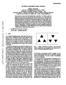
and use Gaussian noise. Since the fraction of unrecovered balls p can be arbitrarily small, in the simulations, we simply define a successful recovery as the cases when all non-zero components are correctly found up to a global phase. In all the simulations, we set P = 5 log(n), d = 15, M = 8K, Lm = 3, Lp = 6, and ε = 1.

0.2 1.04 1.68 2.32 2.96 3.60 4.24 4.88 5.52 6.16 6.80 5 number of measurements/10

0

Figure 2: Probability of successful recovery. We choose n = 220 and K = 50. Different values of Q and SNR are tested, and for each set of parameters, 1000 experiments are conducted.

1/3

(sec )

1/3

0.6

0.8

n=1024 n=2048 n=4096

0.4

time cost

time cost (sec)

0.8

0.2 0 0

20

K

40

60

0.7 0.6

K=5 K=10 K=15

0.5 0.4 0.3 10

12

log(n)

14

16

Figure 3: Time cost. We choose Q = 2 log2 (n) and SNR = 20dB. Different values of n and K are tested, and for each set of parameters, 100 experiments are conducted and the average time cost is shown.

In Figure 2, we show the results of simulations on the probability of 11

successful recovery as a function of the number of measurements and the SNR. Since the total number of measurements is dominated by Q. The sample complexity is mainly determined by Q. Therefore, we fixed P , i.e., the size of the test matrix, and tried different values of Q. From the results, we can see that the sublinear scheme can successfully recover the signal at relatively low SNR, such as 16dB, when Q = 2 log2 (n) and the number of measurements is 6.8 × 105 . In Figure 3, we show the results of simulations on the time cost of the sublinear scheme7 . It can be seen that the time cost of sublinear scheme is indeed low and linear in K and Θ(log3 (n)).

Acknowledgment The authors would like to thank Yudong Chen and Xiao Li for helpful discussions.

References [1] R. Pedarsani, K. Lee, and K. Ramchandran, “Phasecode: Fast and efficient compressive phase retrieval based on sparse-graph-codes,” arXiv preprint arXiv:1408.0034, 2014. [2] R. Vershynin, “Introduction to the non-asymptotic analysis of random matrices,” arXiv preprint arXiv:1011.3027, 2010. [3] E. J. Candes, T. Strohmer, and V. Voroninski, “Phaselift: Exact and stable signal recovery from magnitude measurements via convex programming,” Communications on Pure and Applied Mathematics, vol. 66, no. 8, pp. 1241–1274, 2013. [4] B. Alexeev, A. S. Bandeira, M. Fickus, and D. G. Mixon, “Phase retrieval with polarization,” SIAM Journal on Imaging Sciences, vol. 7, no. 1, pp. 35–66, 2014. [5] H. Ohlsson, A. Y. Yang, R. Dong, and S. S. Sastry, “Compressive phase retrieval from squared output measurements via semidefinite programming,” arXiv preprint arxiv.org/abs/1111.6323, 2011. 7

The simulations are conducted on a laptop with 2.8 GHz Intel Core i7 CPU and 16 GB memory.

12

[6] O. Bunk, A. Diaz, F. Pfeiffer, C. David, B. Schmitt, D. K. Satapathy, and J. F. van der Veen, “Diffractive imaging for periodic samples: retrieving one-dimensional concentration profiles across microfluidic channels,” Acta Crystallographica Section A: Foundations of Crystallography, vol. 63, no. 4, pp. 306–314, 2007. [7] E. G. Loewen and E. Popov, Diffraction gratings and applications. CRC Press, 1997. [8] M. Mirhosseini, O. S. Maga˜ na-Loaiza, S. M. H. Rafsanjani, and R. W. Boyd, “Compressive direct measurement of the quantum wavefunction,” arXiv preprint arXiv:1404.2680, 2014. [9] D. J. Love, R. W. Heath, W. Santipach, and M. L. Honig, “What is the value of limited feedback for mimo channels?” Communications Magazine, IEEE, vol. 42, no. 10, pp. 54–59, 2004. [10] J. C. Candy, “A use of limit cycle oscillations to obtain robust analogto-digital converters,” Communications, IEEE Transactions on, vol. 22, no. 3, pp. 298–305, 1974. [11] T. Richardson and R. Urbanke, Modern coding theory. University Press, 2008.

Cambridge

[12] X. Li, S. Pawar, and K. Ramchandran, “Sub-linear time support recovery for compressed sensing using sparse-graph codes,” arXiv preprint arXiv:1412.7646, 2014. [13] S. Pawar and K. Ramchandran, “Computing a k-sparse n-length discrete fourier transform using at most 4k samples and o (k log k) complexity,” arXiv preprint arXiv:1305.0870, 2013. [14] I. Waldspurger, A. d’Aspremont, and S. Mallat, “Phase recovery, maxcut and complex semidenite programming,” Mathematical Programming, pp., pp. 1–35, 2013. [15] X. Li and V. Voroninski, “Sparse signal recovery from quadratic measurements via convex programming,” arXiv preprints arXiv:1209.4785, 2012. [16] K. Jaganathan, S. Oymak, and B. Hassibi, “Sparse phase retrieval: Convex algorithms and limitations,” pp. 1022–1026, 2013.

13

[17] ——, “Phase retrieval for sparse signals using rank minimization,” in Proceedings of IEEE International Conference on Acoustics, Speech and Signal Processing, 2012, pp. 3449–3452. [18] R. Gerchberg and W. Saxton, “Phase determination for image and diffraction plane pictures in the electron microscope,” Optik, vol. 34, pp. 275–284, 1971. [19] P. Netrapalli, P. Jain, and S. Sanghavi, “Phase retrieval using alternating minimization,” arXiv preprints arXiv:1306.0160, 2013. [20] E. Candes, X. Li, and M. Soltanolkotabi, “Phase retrieval via wirtinger flow: Theory and algorithms,” arXiv preprint arXiv:1407.1065, 2014. [21] Y. Chen, X. Yi, and C. Caramanis, “A convex formulation for mixed regression with two components: Minimax optimal rates,” in Proceedings of The 27th Conference on Learning Theory, 2014, pp. 560–604. [22] A. C. Gilbert, M. J. Strauss, J. A. Tropp, and R. Vershynin, “Algorithmic linear dimension reduction in the ℓ1 norm for sparse vectors,” arXiv preprint cs/0608079, 2006. [23] S. Pawar, “Pulse: Peeling-based ultra-low complexity algorithms for sparse signal estimation,” Ph.D. dissertation, PhD Dissertation, 2013. [24] M. Rudelson and R. Vershynin, “Hanson-wright inequality and subgaussian concentration,” arXiv preprint arXiv:1306.2872, 2013.

14

Appendix A

Notations

We introduce some useful notations for the proofs. Here, k · kF denotes the Frobenius norm of a matrix, k·k denotes the operator norm of a matrix. For a sub-exponential random variable, k · kψ 1 denotes the sub-exponential norm of it; for a sub-gaussian random variable, k · kψ2 denotes the sub-gaussian norm of it [2]. The notations c, ci , C, and Ci represent absolute constants with positive value. In our model, we also assume that the noise wi satisfies E[|wi |] = µ, E[wi2 ] = σ 2 , and kwi kψ1 = ν. Since the entries in A0 and F 0 are bounded and thus sub-gaussian, we let η = k |aij | kψ2 and η0 = k |f0,ij | kψ2 , where aij and f0,ij are entries of A0 and F 0 .

B

Proof of Theorem 1

In order to prove Theorem 1, we need to prove Lemma 1 first. Here we restate Lemma 1 with more details. Lemma 1. There exists ζ > 0, determined by η, ν, and σ, such that when φ > µ/ζ, for any t0 ∈ (µ, ζφ),   1 kwk1 ≥ t0 = O(1/n2 ), (7) P P and P ˆ ≁ x. when x



1 P



H 2 ˆ < t y − A(ˆ x x )

0 = O(1/n ), 1

(8)

See the proof of Lemma 1 in Appendix C. Now we can analyze the failure probability of the almost-linear scheme. Since the bipartite graph is d-left regular, there are dn balls in all the bins. In the first iteration, we need to search all the balls. For each ball, we need to check Θ(1) possible magnitudes. Therefore, we need to do Θ(n) tests in the first iteration (d is also a constant). Similarly, in the later iterations, we need to do at most Θ(n) tests. Since it is proved in [1] that the number of iterations is a constant, we need to do Nt = Θ(n) tests. Lemma 1 tells us that, for any energy test, if the tests before it are all correct, and thus we have the correct colored balls, then, the error probability of this test is O(1/n2 ). More specifically, let Ei 15

be the event that there is an error in the ith test, while the tests 1, . . . , i − 1 are all correct. The event Etest that there is error in all the energy tests can be decomposed as Nt [ Ei . Etest = i=1

By union bound, we have

P {Etest } ≤ Nt

Nt X i=1

P {Ei } = Θ(n)O(1/n2 ) = O(1/n).

Another possibility of making an error lies in the ball coloring algorithm itself. When there is no error in energy tests, this probability is O(1/K) as analyzed in the noiseless case. Therefore the failure probability of the almost-linear scheme is ∁ ∁ } P {Ea } = P {Ea |Etest } P {Etest } + P{Ea |Etest }P{Etest ∁ ≤ P {Etest } + P{Ea |Etest }

= P {Etest } + P {Ecoloring } = O(1/n) + O(1/K) = O(1/K)

The sample and computational complexity are already analyzed in Section 4. Now we complete the proof.

C

Proof of Lemma 1

To prove equation (7), we simply use the Bernstein’s inequality in [2]. For any t > 0, ) ( P 1 X (|wi | − E [|wi |]) > t P P i=1   2  t t , . ≤ exp −C1 P min ν2 ν Therefore, by choosing t0 > E [|wi |] = µ and t = t0 − µ, we have   1 P kwk1 ≥ t0 ≤ exp [−δ1 P ] . P 16

Since δ1 is a constant and P = Θ(log(n)), equation (7) is proved. Now we prove equation (8). Before getting into the details of the proof, we give the definition of a new notation φ. For two vectors p, q ∈ Sn , it is easy to see that p ≁ q ⇔ ppH − qq H 6= 0. Since the entries of p and q lie in the quantized set S, we know that there exists φ > 0, such that kppH − qq H kF > φ, when p ≁ q, where φ depends on ε, Lm , and Lp . Then, we need the following lemma. H Lemma 3. Given two vectors x1 , x2 ∈ CN , let X = x1 xH 1 − x2 x2 6= 0. A is the linear function defined in (3), and w is the noise. Then, for any s > 0, we have,   1 kA(X) + wk1 < (ζ − sηd ) kXkF − 2sν P P   ≤ exp −C0 P min {s2 , s} ,

where ζ > 0 depends on η, σ, and ν, ηd > 0 only depends on η.

ˆ H) = See the proof of Lemma 3 in Appendix D. Note that y − A(ˆ xx H H H H ˆx ˆ ) + w, and that kxx − x ˆx ˆ kF > φ. Now using Lemma 3, A(xx − x conditioning on h, we have for any s > 0,  

1 H ˆ ) < ζφ − (ηd φ + 2ν)s | h P xx

y − A(ˆ P 1   2 ≤ exp −C0 P min {s , s} . (9)

Since (9) holds for any h, we know that it also holds without conditioning 0 , then on h. If ζφ > t0 , we can choose s = ηζφ−t d φ+2ν P





1

H ˆ ) < t0 ≤ exp [−δ2 P ] . xx

y − A(ˆ P 1

Since δ2 is a constant and P = Θ(log(n)), equation (8) is proved. Then, we can conclude that there exists ζ, determined by the statistics of noise, such that when φ > µ/ζ, for any threshold t0 ∈ (µ, ζφ), the energy test fails with probability O(1/n2 ). This completes the proof of Lemma 1.

D

Proof of Lemma 3

The proof of Lemma 3 is based on similar ideas appeared in [21]. Let ξ = A(X) + w, then ξi = aH i Xai + wi . According to the definition of the 17

matrix A, we know that the Hanson-Wright inequality for complex random variables in Appendix G holds for aH i Xai and we have for every t > 0,    H P aH i Xai − E ai Xai > t " ( )# t2 t ≤6 exp −c min , η 4 kXk2F η 2 kXk    1 t t − , 2 ≤6 exp −c min η 2 kXkF 4 η kXkF    t 1 − 2 ≤6 exp c , 4 η kXkF where the second inequality is due to the fact that (a − 1/2)2 ≥ 0 and H kXk ≤ kXkF . From [2], we know that aH i Xai − E ai Xai is a subexponential random variable with sub-exponential norm

H   2

ai Xai − E aH

(10) i Xai ψ1 ≤ Cη kXkF .

On the other hand,

 H  E ai Xai = 1 kx1 k2 − kx2 k2 ≤ 1 kXk . F 2 2 2 2

Thus, it gives us

   H  H

kξi kψ1 = aH i Xai − E ai Xai + E ai Xai + wi ψ1  H

H    H ≤ ai Xai − E ai Xai ψ1 + E ai Xai + ν ≤(Cη 2 + 1/2) kXkF + ν,

(11)

 H  where  Hthe first  inequality  H is due  to the fact that E ai Xai is a constant, kE ai Xai kψ1 = |E ai Xai |, and that kwi kψ1 = ν. Then k|ξi | − E [|ξi |]kψ1 ≤ 2 kξi kψ1 ≤ ηd kXkF + 2ν,

(12)

where ηd = 2Cη 2 + 1. Now according to Bernstein’s inequality in [2], we have for every t > 0, ) ( P 1 X (|ξi | − E [|ξi |]) < −t P P i=1    t t2 , . ≤ exp −C0 P min (ηd kXkF + 2ν)2 ηd kXkF + 2ν 18

Let t = s(ηd kXkF + 2ν). For any s > 0, ( ) P 1 X P (|ξi | − E [|ξi |]) < −s(ηd kXkF + 2ν) P i=1   ≤ exp −C0 P min {s2 , s} .

(13)

By Cauchy-Schwartz inequality, for any i ∈ [P ], we have q     i h  2 
2 3 E ξi ≤ E [|ξi |] E |ξi | ≤ E [|ξi |] E ξi2 E ξi4 , which implies

E [|ξi |] ≥

s

  (E ξi2 )3   . E ξi4

(14)

According to the definition of sub-exponential norm and the fact that ηd > 1, we have   E ξi4 ≤ (4 kξi kψ1 )4 ≤ (2ηd kXkF + 4ν)4 ≤ (8ηd2 kXk2F + 32ν 2 )2 .

On the other hand, we have      2 2 E ξi2 = E (aH i Xai ) + E wi
  H + σ2 = E (aH i Xai )tr ai ai X
  H + σ2 = E tr (aH i Xai )ai ai X  
H 2 = tr E (aH i Xai )ai ai X + σ 1 = tr ((X + tr (X) I)X) + σ 2 4 1 ≥ kXk2F + σ 2 . 4

(15)

(16) (17)

H Here we give an explanation of equation (16). Let Y = (aH i Xai )ai ai . Then,

E [Yjk ]   X =E  a∗ig Xgh aih aij a∗ik  1≤g,h≤n

=

n X g=1

  X  ∗  E a∗ig Xgg aig aij a∗ik + E aig Xgh aih aij a∗ik . g6=h

19

If j = k, we have E[Yjj ] =

n X g=1

Xgg E[|aig |2 |aij |2 ] +

1 = (tr (X) + Xjj ). 4

X

Xgh E[a∗ig aih |aij |2 ]

X

Xgh E[a∗ig aih aij a∗ik ]

g6=h

If j 6= k, we have E[Yjk ] =

n X g=1

Xgg E[|aig |2 aij a∗ik ] + 2

2

= Xjk E[|aij | |aik | ] 1 = Xjk . 4

g6=h

Therefore, E[Y ] = 41 (X + tr (X) I). By combining (14), (15), and (17), we have v !2  u  2 1 u 2 kXk + σ 1 2 F t 4 2 kXkF + σ E [|ξi |] ≥ 4 8ηd2 kXk2F + 32ν 2

≥ ζ kXkF , n o 1 σ2 where ζ = 12 min 32η is a constant determined by the distribution 2 , 32ν 2 d

of aij and wi . Then according to (13), we have ) ( P 1 X |ξi | < ζ kXkF − s(ηd kXkF + 2ν) P P i=1   ≤ exp −C0 P min {s2 , s} ,

which completes the proof.

E

Proof of Theorem 2

To prove Theorem 2, we need to use Lemma 2. Here, we restate Lemma 2, providing more details. Lemma 2. If Ts = 1, supp(xs ) = {ls }, and threshold t1 ∈ (0, ε2 /2), then for any j ∈ [R], o n P ˜bj 6= bjls = O(1/K 3 ). 20

See the proof of Lemma 2 in Appendix F. Then, by union bound, we ˜ 6= B l } = O(R/K 3 ) ≤ O(1/K 2 ), since K = βnδ . Now we know that P{b s can see that we can reliably find ls from the measurements with probability 1 − O(1/K 2 ). For a bin with Ts = 1, the probabilities of error in index tests and energy test are O(1/K 2 ) and O(1/n2 ), respectively. Therefore, the error probability of the tests for this bin is O(1/K 2 ). For a bin with Ts > 1, only the energy test should be considered and its error probability is O(1/n2 ). Then, we know the probability of making mistakes in the index and energy tests is O(1/K 2 ). Since there are Θ(K) bins and a constant number of iterations, using the same decomposition method as in the proof of Theorem 1, we know that the error probability of all the tests is O(1/K). Similar to the almost-linear scheme, considering the O(1/K) probability of incomplete recovery in the ball coloring algorithm when there is no error in the index and energy tests, the failure probability of sublinear scheme is P{Es } = O(1/K). Since the sample and computational complexity are already analyzed in Section 5, the proof of Theorem 2 is now complete.

F

Proof of Lemma 2

First, we define an event Eh such that there are more than C3 log K active balls in a bin. As mentioned in [23], we have P{Eh } = O(1/K 3 ). Now we condition on the coding pattern h such that Eh∁ happens, and thus |supp(x)| = T ≤ C3 log K. Similar to the almost-linear algorithm, we define R + 1 linear mappings, A0 , A1 , . . . , AR , where A0 : X 7→ {aH i Xai }i∈[P ] , Aj : X 7→ {f H j,i Xf j,i }i∈[Q] , for j ∈ [R].

Then, We have y j = Aj (xxH ) + wj , j ∈ {0} ∪ [R]. H H ˜ = {X ˜ ij }N ×N := xxH − x ˜ cx ˜H Define the matrix X c = xx − xc xc . Then H ˜ ˜ ˜ j = Aj (X) + wj . There is y˜j,i = f j,i Xf j,i + wj,i . Let fj,i,m be the mth y element of f j,i . Since for a fixed j, fj,i,m’s are independent, using the similar argument in Appendix D, we know that

h i

H ˜

H ˜ 2 ˜

f j,i Xf j,i − E f j,i Xf j,i ≤ C2 η0 X . ψ1

F

˜ F + ν. Since there are 2T − Then we have k˜ yj,i − E[˜ yj,i ]kψ1 ≤ C2 η02 kXk √ ˜ ˜ We also have 1 nonzero entries in X, we have kXkF ≤ 2T − 1Lm ε. √ T√ ≤ C3 log K, therefore we have k˜ yj,i − E[˜ yj,i ]kψ1 ≤ C4 η02 Lm ε log K + ν ≤ ζ0 log K, where ζ0 is determined by η0 , Lm , ε, and ν. 21

˜ only has one On the other hand, since Ts = 1 and supp(xs ) = {ls }, X 2 ˜ yj,i ] = nonzero element on the diagonal, i.e., Xls ls = |xls | . We have E[˜ E[|fj,i,ls |2 ]|xls |2 = bjls |xls |2 . According to Bernstein’s inequality, for every t ≥ 0, we have ) ( Q 1 X 2 (˜ yj,i − bjls |xls | ) > t | h P Q i=1    t2 t ≤2 exp −C5 Q min , √ ζ02 log K ζ0 log K   2 C5 p ≤2 exp − 2 Q min t , t , ζ0 where the last inequality comes from the fact that Q = Θ(log2 N ). Now choose t1 = t < ε2 /2. When bjls = 0, we know that ) ( Q 1 X y˜j,i > t1 | h P Q i=1   2 C5 p ≤2 exp − 2 Q min t1 , t1 , ζ0

(18)

and when bjls = 1, we have

) ( Q 1 X y˜j,i < t1 | h P Q i=1 ) ( Q 1 X y˜j,i < t1 | h ≤P Q i=1 ) ( Q 1 X ≤P y˜j,i < |xls |2 − t1 | h Q i=1 ) ( Q 1 X 2 y˜j,i − |xls | > t1 | h ≤P Q i=1   2 C5 p ≤2 exp − 2 Q min t1 , t1 , ζ0

(19)

(20)

where the inequality (19) is due to thePfact that t1 < ε2 /2 and |xls |2 ≥ ε2 . ˜j,i| > t1 }, when bjls = 0, and Define the error events Eindex = {| Q1 Q i=1 y 22

Eindex = {| Q1

PQ

˜j,i| i=1 y

< t1 }, when bjls = 1. Then, since Q = Θ(log2 (n))

and inequalities (18) and (20) hold for any h ∈ Eh∁ , we have, P{Eindex |Eh∁ } = O(1/K 3 ). Now we know that

P{Eindex } = P{Eindex |Eh∁ }P{Eh∁ } + P{Eindex |Eh }P{Eh } ≤ P{Eindex |Eh∁ } + P{Eh }

= O(1/K 3 ) + O(1/K 3 )

= O(1/K 3 ), which completes the proof.

G

Hanson-Wright Inequality for Complex Random Variables

Theorem 3. Let γ = {γi }i∈[n] ∈ Cn be a random vector with independent entries γi , satisfying E [γi ] = 0, and |γi | is sub-gaussian with k|γi |kψ2 ≤ η for all i ∈ [n]. Let U ∈ Cn×n be a Hermitian matrix. Then, for every t ≥ 0,    P γ H U γ − E γ H U γ > t " ( )# t t2 , ≤6 exp −c0 min . η 4 kU k2F η 2 kU k Proof. Let α = {αi }i∈[n] and β = {βi }i∈[n] be the real and imaginary parts of γ. Then, we know that αi ’s and βi ’s are sub-gaussian random variables with kαi kψ2 ≤ η and kβi kψ2 ≤ η for all i ∈ [n]. Note that here, although γi ’s are independent, the real and imaginary parts of γi are not necessarily independent for a certain i. In other words, for any i, αi and βi may not be independent. Let V and W be the real and imaginary parts of U . Since U is a Hermitian matrix, we have V = V T and W = −W T . We also know that γ H U γ is a real number. Then, we have γ H U γ = αT V α − 2αT W β + β T V β.

23

   Therefore, P γ H U γ − E γ H U γ > t is upper bounded by three terms,    P γ H U γ − E γ H U γ > t    ≤P αT V α − E αT V α > t/4    +P αT W β − E αT W β > t/4    +P β T V β − E β T V β > t/4 .

(21)

Since αi ’s are independent and E [αi ] = 0, according to the Hanson-Wright inequality for real numbers [24], we have    P αT V α − E αT V α > t/4 " ( )# t t2 , ≤2 exp −c1 min . η 4 kV k2F η 2 kV k We also have kV kF ≤ kU kF , kV k ≤ kU k. Therefore,    P αT V α − E αT V α > t/4 )# " ( t t2 . ≤2 exp −c1 min , η 4 kU k2F η 2 kU k

(22)

And similarly,    P β T V β − E β T V β > t/4 " ( )# t2 t ≤2 exp −c2 min . , η 4 kU k2F η 2 kU k

(23)

Now consider the cross term. Let Wij be the entries P of W . Since W = −W T , Wii = 0 for all i ∈ [n]. Then we have αT W β = i6=j Wij αi βj , and    E αT W β = 0. Then, we can bound P αT W β > t/4 in the same way as in [24]. We have  P αT W β > t/4 )# " ( t2 t . (24) ≤2 exp −c3 min , η 4 kU k2F η 2 kU k By combining (22), (23), and (24), Theorem 3 is proved.

24