Oct 10, 2007 - Abstract. To repeatedly evaluate linear combinations of box-splines in a fast and stable way, in particular along knot planes, we convert to and ...
Fast and stable evaluation of box-splines via the B´ezier form Minho Kim and J¨org Peters October 10, 2007 Abstract To repeatedly evaluate linear combinations of box-splines in a fast and stable way, in particular along knot planes, we convert to and tabulate the box-spline as piecewise polynomials in B´ezier form. We show that the B´ezier coefficients can be stored as integers and a rational scale factor and derive a hash table for efficiently accessing the B´ezier pieces. The preprocessing, the resulting evaluation algorithm and use in a widely available ray-tracing package are illustrated for splines based on two trivariate box-splines, the 7-direction box-spline on the Cartesian lattice and the 6-direction box-spline on the FCC lattice.
1
Introduction
As a generalization of the univariate uniform B-spline to multivariate shiftinvariant lattices, box-splines are useful in many applications. For example, they can be used to create a continuous field from data sampled at the lattice points. This reconstruction typically uses quasi-interpolation or outright interpolation and requires exact values of the box splines. But evaluation on lattice edges and faces, a likely operation for a field so constructed, requires care. Already de Boor [5] and later Kobbelt [12] observed a fundamental combinatorial challenge due to the inclusion or exclusion of certain knot planes (Section 3.1.5) and dealt with it in two different ways in their respective recursive box-spline evaluation algorithms. Our interest was piked by the example of Figure 1a, where the algorithm of [12] fails due to subtle numerical round-off in the underlying MATLAB® routine. An alternative approach to direct recursion is to evaluate after conversion to the B´ezier form. This approach was pioneered by Chui and Lai [2, 13] in two variables, and recently by Casciola et al. [1] for a class of trivariate box-splines. Since any spline is a linear combination of shifts of one or more box-splines, we focus attention on the box-spline basis (or generator) functions. The point of the conversion is that the total degree B´ezier form of the polynomial pieces 1
(a)
(b)
Figure 1: Isosurfaces for 10−1 (blue), 10−2 (green), 10−3 (red) and 10−10 (purple) of the 6-direction box-spline basis function (Section 6.2), (a) evaluated by [12] and (b) the correct isosurface. (Section 3.2.1) has a stable evaluation algorithm exactly on the knot planes where the recursive algorithms encounter its challenges. In fact, de Casteljau’s algorithm is even of lower complexity along knot planes. The key challenge for this approach are the derivation and exact representation of the change of basis. Our first contribution, generalizing [13, 1], is Theorem 1: (1) the B´ezier coefficients, expressing a box-spline with integer directions, are rational. This allows us to use a simple interpolation-based approach for deriving a change-of-basis matrix with exact integer entries, scaled by a rational number. While both the recursive and the conversion approach benefit from localization, i.e. from determining what box-splines influence the evaluation, the conversion approach must efficiently determine the simplex of B´ezier evaluation. This forces an understanding of the decomposition of the domain by the knot planes implied by the box-spline directions. Our second contribution is (2) an indexing strategy, based on the box-spline directions, for finding the simplex of B´ezier evaluation for a given parameter (Section 4.1). The one-time pre-resolution of the combinatorics of the box-splines required by the indexing strategy is at the core of improved speed, by orders of magnitude (Table 3), compared to evaluators that resolve the combinatorics at run time. Conversion plus indexing, both pre-computed, stored and quickly accessed, yield an (3) algorithm for fast evaluation of splines based on box-splines that is stable, in particular along knot planes (Algorithm 5.1).
2
2
Review of Existing Evaluation Techniques
Two different MATLAB® packages for evaluating box-splines, [5] and [12], are based on the recursive formula (3). These packages, which are freely available from the Internet, and immensely useful, because they accommodate arbitrary matrices Ξ and they are well-explained in their companion papers. As the papers point out, evaluators based on recursion face a key difficulty when evaluating a combination of shifts of the characteristic function. Unless the combinatorics on inclusion and exclusion of knot planes are correctly and consistently addressed, evaluation along knot planes yield incorrect results. If the evaluation is correct, it is called ‘stable’. De Boor [5] addresses the stability problem by perturbing input points that are deemed too close to knot planes. Kobbelt [12] untangles the combinatorics explicitly by deferring translation of input points until the base level of the recursion to avoid round-off. This algorithm also pre-computes the normals of the knot planes in a deterministic way to avoid that a knot plane is doubly included or completely excluded by two adjacent characteristic functions. We found that [12] works well for bivariate box-splines, but the released code fails in higher dimensions as the example in Figure 1a illustrates. After analyzing the problem in more detail than we had intended, we found the flaw in the application of the MATLAB® null function call. Generically, the null space is determined by Singular Vector Decomposition [14]. But even minute SVD round-off errors create instability. Tellingly, we were often able to remove the instability, in the trivariate cases we tested, by adding the ’r’ parameter to the null function call, i.e. by enforcing close-to-rational representation via Gaussian elimination. The algorithms of Jetter and McCool [11, 15] approximate box-splines by sampling in the Fourier domain and applying inverse FFT. This way, they leverage the closed form of box-splines in the Fourier domain. Explicit formulas for the conversion of box-splines to B´ezier representation have been derived by Chui and Lai [2, 13] in two variables and by Casciola et al. [1] for a class of trivariate box-splines. The approach of [2] generates the B´ezier form of bivariate box-splines by comparing directional derivatives of box-splines with those of the B´ezier form. Applying this approach to 3- and 4-direction bivariate box-splines, [13] provides explicit Fortran codes and shows that the B´ezier coefficients are rational. Similarly, [1] converts the important class of trivariate box-splines spanned by four directions. Condat and van de Ville [3] based the evaluation of bivariate 3-direction boxsplines on reduction of the box-splines to cone splines, i.e. truncated powers. Dæhlen [10] went one step further by converting the cone splines to simplex splines of one dimension lower. The approach is shown to be efficient for bivariate box-splines and, with explicit guidance along knot lines, for the 4-direction trivariate box-spline. Except for [11], where the goal is interpolation, all the above aim at evaluating 3
individual box-splines. Splines in box-spline form would off hand be evaluated by evaluating shifts of the underlying box-splines individually, and then adding their contribution weighted by the coefficients.
3
Box-splines and the B´ ezier form
In Section 3.1, we briefly review the basic definitions and properties of boxsplines and in Section 3.2, we review the multivariate polynomials in B´ezier form. In Section 3.3, we prove that the B´ezier coefficients of the polynomial pieces of a box-spline with integer directions are rational.
3.1
Box-splines
We use the notation made standard by the ‘box-spline book’ [6]. Here ‘boxspline’ denotes a smooth piecewise polynomial of finite support. A spline is a linear combinations of shifts of a box-spline. If the shifts of a box-spline are linearly independent, the box-spline is a basis function. 3.1.1
Definition
Geometrically, the value of a box-spline with direction matrix Ξ ∈ Rs×n at x ∈ ranΞ ⊂ Rs is the shadow-density [6] (I-3) � MΞ (x) := voln−dim ranΞ Ξ−1 {x} ∩ /| det Ξ|,
i.e. the scaled volume of the intersection of a cube ⊂ Rn , n ≥ s, with the preimage Ξ−1 {x} of x, an (n−dim ranΞ)-dimensional subspace in Rn . The cube or box gives the box-spline its name. In more detail,
:= [0..1)n is an n-dimensional half-open unit cube,
Ξ is the s × n direction matrix, possibly with repeated columns, of the box-spline MΞ (Section 6.1 gives an example), ranΞ is the subspace spanned by the column vectors {ξ : ξ ∈ Ξ}, Ξ−1 (x) is the preimage of x when viewing Ξ as a linear transformation Ξ : Rn → Rs and vold (·) is the d-dimensional volume of its argument.
In the following, we assume dim ranΞ = s.
4
3.1.2
Degree and Continuity
A box-spline MΞ is a piecewise polynomial on ranΞ. Its degree is less than or equal to k := k(Ξ) := #Ξ − s where #Ξ denotes the number of columns in Ξ. The polynomial pieces join to form a function in C m−1 (ranΞ) where [6] (p.9) m := m(Ξ) := min{#Z : Z ∈ A(Ξ)} − 1 and [6] (p.8) A(Ξ) := {Z ⊆ Ξ : Ξ\Z does not span}. 3.1.3
Spline Space
A spline fΞ spanned by a box-spline MΞ is an infinite linear combination of the shifts of the box-splines on the integer grid [6] (p.33): X fΞ := M (· − j)a(j) (1) j∈Zs
where a : Zs → R is a mesh function that returns the coefficient corresponding to a mesh location. 3.1.4
Differentiation
With DZ := Πζ∈Z Dζ a composition of differential operators Dζ := and
Ps
ν=1
ζ(ν)Dν
∇Z := Πζ∈Z ∇ζ a composition of backward difference operators such that ∇ζ φ := φ − φ(· − ζ),
a derivative of MΞ in the directions Z ⊆ Ξ equals the backward difference of MΞ\Z along them [6] (I-30): DZ MΞ = ∇Z MΞ\Z . 3.1.5
Knot Planes
According to [6] (I-37), a box-spline is a piecewise polynomial with pieces delineated by a shift-invariant mesh on Zs generated by the collection of knot planes (hyperplanes spanned by columns of Ξ) H(Ξ) [6] (p.16): [ H + Zs . (2) Γ(Ξ) := H∈H(Ξ)
The mesh Γ(Ξ) decomposes Rs into convex polytopes. 5
3.1.6
Recurrence Relation
As long as MΞ\ξ for ξ ∈ Ξ is continuous at x = Ξt ∈ Rs , t ∈ Rn , the box-spline MΞ can be evaluated recursively with the recurrence [6] (I-43): X (n − d)MΞ (x) = tξ MΞ\ξ (x) + (1 − tξ )MΞ\ξ (x − ξ). (3) ξ∈Ξ
Here tξ is the component of the vector t associated with the column ξ ∈ Ξ by x = Ξt. 3.1.7
Change of Variables
Using [6] (I-23), given an invertible linear transformation X ∈ Rs×s , one can show that splines spanned by MΞ on the grid X −1 Zs can be expressed as splines spanned by MXΞ on the integer grid Zs : X X MΞ (· − j) b(j) = | det X| MXΞ (X · −j) b(X −1 j) (4) j∈Zs
j∈X −1 Zs
where b : X −1 Zs → R is a mesh function that returns the coefficient corresponding to a mesh location.
3.2 3.2.1
The B´ ezier Form of a Multivariate Polynomial Definition
Let {vj ∈ Rs : j ∈ {1, ..., s + 1}} be a collection of vertices of a non-degenerate simplex σ. The map �−1 � � � x v1 · · · vs+1 s s+1 βσ : R → R : x 7→ (5) 1 ··· 1 1 is called the barycentric coordinate function with respect to σ [4]. The B´ezier form of an s-variate polynomial of total degree d and coefficients c := {cα ∈ R : |α| = d, α ∈ Z+ s+1 } defined on σ, is a polynomial X cα bdα (u) P (u) := |α|=d
where u is in barycentric coordinates w.r.t. σ, Ps+1 |α| := i=1 α(i), � αd := Πs+1d!α(i)! , i=1
6
uα := Πsi=1 u(i)α(i) and � {bdα (u) := αd uα : |α| = d} are the Bernstein basis polynomials of degree d.
Denote the j-th unit vector by ij . Then bdα (ij ) = 1 if α = dij and zero otherwise. Therefore, P |vj = P (ij ) = cdij . In other words, the B´ezier form of a multivariate polynomial interpolates its vertex coefficients {cα : α = dij , j ∈ {1, ..., s + 1}}. 3.2.2
Differentiation
The directional derivative of P along one of the edges of σ is X X (cβ+ii − cβ+ij )bβd−1 . cα bdα = d Dvi −vj P = Dvi −vj
3.3
(6)
|β|=d−1
|α|=d
Rationality of box-splines in B´ ezier Form
In [13], Lai proved for 3- and 4-direction bivariate box-splines and in [1] Casciola et al. proved for 4-direction trivariate box-splines that the coefficients for those box-splines in B´ezier form are rational numbers. In this section, we generalize this observation. We start by observing that rationality is preserved by box-splines with rational direction matrices. Lemma 1. Let Ξ ∈ Qs×n and rank(Ξ) = s. If x ∈ Qs then MΞ (x) ∈ Q. Proof. We use induction on #Ξ. Let Ξ ∈ Qs×s . Then 1/| det Ξ| ∈ Q and MΞ (x) = χΞ /| det Ξ| ∈ Q where χΞ is the characteristic function on Ξ , a linear transformation of the unit cube . Now assume the claim holds for MΞ\ξ . That is MΞ\ξ (x) ∈ Q and MΞ\ξ (x − ξ) ∈ Q since x − ξ ∈ Qs . Since rank(Ξ) = s, there exists an invertible submatrix ′ s×s Ξ of Ξ. Since Ξ′−1 ∈ Qs×s , there also exists t ∈ Qn so that x = Ξt = P∈ Q ξ∈Ξ tξ ξ. The recursion (3), (n − s)MΞ (x) =
X
tξ MΞ\ξ (x) + (1 − tξ )MΞ\ξ (x − ξ),
ξ∈Ξ
then implies that MΞ (x) ∈ Q. Now denote by Γ(Ξ) the collection of all shifts of (s-1)-dimensional hyperplanes spanned by columns of Ξ (Equation (2)). Each Hi ∈ Γ(Ξ) is defined by a
7
plane equation nTi (· − ji ) = 0. We denote by knot-vertex the intersection x of s hyperplanes H1 , · · · , Hs ∈ Γ(Ξ) whose normals span Rs : T T n1 n1 j1 .. .. −1 x = N η, where N := . and η := . . (7) nTs
nTs js
Lemma 2. Let Ξ ∈ Qs×n and rank(Ξ) = s. Then the polynomial pieces of MΞ can be represented in B´ezier form with vertex coefficients in Q.
Proof. By Section 3.1.5, the piecewise polynomials of MΞ can be expressed over convex polytopes delineated by knot planes with rational normals. Since Ξ ∈ Qs×n , we have ni ∈ Qs and hence N −1 ∈ Qs×s . Since the shifts are on the integer grid, ji ∈ Zs , and therefore all knot-vertices are in Qs . Since any s-dimensional convex polytope can be decomposed into s-dimensional simplices without introducing any new vertex, the claim follows from Lemma 1. Lemma 2 can be extended to the main conclusion. Theorem 1. Let Ξ ∈ Zs×n and rank(Ξ) = s. Then the polynomial pieces of MΞ can be represented in B´ezier form with coefficients in Q. Proof. We use induction on #Ξ. If Ξ ∈ Zs×s , then the B´ezier polynomial is constant and equals the value at the vertex. By Lemma 2, this value is rational. Since rank(Ξ) = s, for any w ∈ Qs there exists an y ∈ Qn so that w = Ξy = P ξ∈Ξ yξ ξ. By linearity of differentiation and [6] (I-30), X X Dw M Ξ = yξ Dξ M Ξ = yξ ∇ξ MΞ\ξ . ξ∈Ξ
ξ∈Ξ
By the induction hypothesis, MΞ\ξ is in piecewise B´ezier form with coefficients in Q. And, since the knot planes are invariant under integer shifts and Ξ ∈ Zs×n , ∇ξ MΞ\ξ is a difference of B´ezier polynomials with coefficients in Q. Therefore Dw MΞ is in piecewise B´ezier form with coefficients in Q.
Now let vi and vj be any two knot-vertices of a simplex (possibly obtained by decomposition of an s-dimensional convex polytope. Then w := vi −vj ∈ Qs and Dvi −vj MΞ has rational coefficients, i.e., in the notation of (6), (cβ+ii − cβ+ij ) ∈ Qs . Since the vertex coefficients are rational by Lemma 2, rationality of the differences propagates rationality to all B´ezier coefficients {cα }.
4
Preprocessing box-splines
We first discuss how to encode (or index) the total degree B´ezier domain simplices for a particular direction matrix Ξ and then how to find the changeof-basis for conversion of box-splines to the B´ezier form. We note that the 8
combinatorial work of defining the partition into domain simplices of B´ezier pieces is done only once ever per box-spline generator or basis function since the result is tabulated and quickly accessed by the following indexing strategy.
4.1
Indexing a Simplex
Unless the directions form a tensor-product, the most convenient representation of the polynomial pieces of a box-spline is the B´ezier form on a simplex (Section 3.2.1). The challenge is to smartly index each simplex in suppMΞ to derive, store and efficiently access the B´ezier coefficients. Our decomposition is inspired by BSP (Binary Space Partitioning) trees (see e.g. [9, 16]). Let Γ (Ξ) ⊂ Γ(Ξ) be the set of knot planes of MΞ , each of which splits into two s-dimensional subspaces. Then each path of the tree is converted into a pair of index vectors (i� , i△ ) ∈ Zs × {0, 1}q where q := q(Ξ) := #Γ (Ξ) is the number of knot planes in Γ (Ξ). To start with, we circumscribe the support of the box-spline. Since we assume full rank of Ξ, we may, possibly after change of variables (4), assume that Γ(Ξ) contains all axis-aligned hyperplanes. Let IΞ ∈ Zs be the minimal set of grid points such that suppMΞ ⊂ IΞ + , i.e. IΞ := {j ∈ Zs : (j + ∩suppΞ) 6= ∅}. These cubes are further partitioned into convex polytopes by other knot planes in Γ (Ξ). If the convex polytope is not already a simplex, we have several options, for example decomposition into simplices without adding new vertices. A simple solution is to choose s of the polytope vertices and define the B´ezier polynomial with respect to this (non-degenerate) simplex. de Casteljau’s algorithm may then evaluate outside the simplex. By shift-invariance, each cube is partitioned alike. We now index a simplex by i� ∈ IΞ and i△ ∈ {0, 1}q . In other words, i� identifies a cube intersecting suppΞ and i△ identifies a simplex in that cube. The index vector i△ is computed by membership test against all the knot planes in Γ (Ξ): ( 1, t ≥ 0 i△ (x) := U (NΞ x − ηΞ ), U (t) := (8) 0, t < 0. where NΞ ∈ Qq×s and ηΞ ∈ Qq define the knot planes in Γ (Ξ).
4.2
Computing the Change of Basis
� d+s An s-dimensional B´ezier polynomial of total degree d has coefficients. s � n Since MΞ is of degree n − s, there are s coefficients. And since the B´ezier 9
polynomials are linearly � �independent, we can compute the B´ezier �coefficients by solving the ns by ns linear system obtained by evaluating ns uniformly distributed points in each simplex. We (i) distribute the sample points uniformly so the system is well-formed, (ii) avoid sampling near the knot planes so [12] or [5] evaluate stably, and (iii) choose rational parameters so that Theorem 1 allows us to round to scaled integers by leveraging rational computation in MATLAB®. Typically, box-splines are symmetric and we can reduce the computation and compress the output.
4.3
Barycentric Coordinates
We also pre-compute the matrices in Equation (5) that compute barycentric coordinates u with respect to a simplex {vj } for a point x ∈ Rs in Cartesian coordinates.
5
The Spline Evaluation Algorithm
Given the indexing (hash table), the table of B´ezier coefficients and the precomputed inverse matrices for computing barycentric coordinates, we can evaluate splines, i.e. linear combinations of shifts of box-splines, efficiently and stably. The following algorithm evaluates a spline with box-spline directions Ξ and box-spline coefficients a at a point x. The steps are as follows. First, we find the simplex index i△ of the point x using the membership test (8). We then compute the barycentric coordinates u of x with respect to the simplex. Shifts of the index are used to pick up, via the hash table, all B´ezier coefficients that stem from box-spline shifts whose supports overlap x; and to form their linear combination with weights from a. The coefficients of the resulting B´ezier polynomial are stored in P . Finally, the algorithm evaluates this B´ezier polynomial with coefficient vector P . The following is the pseudocode for spline evaluation. Algorithm 5.1: EvaluateSpline
(a, x)
Ξ
i△ ← U (NΞ (x − ⌊x⌋) − ηΞ ) u ← ComputeBarycentric(i△ , x − ⌊x⌋) P ←
P
i� ∈IΞ
a(⌊x⌋ − i� ) CΞ (i� , i△ )
return EvaluateB´ezier(P, u)
10
Here the subscript Ξ , rather than an argument Ξ, emphasizes that the algorithm requires the pre-processing with respect to Ξ according to Section 4, a(⌊x⌋ − i� ) ∈ R is the box-spline coefficient with index ⌊x⌋ − i� ∈ Zs , x is the input point (in Cartesian coordinates) to be evaluated, NΞ and ηΞ define the knot planes in Γ (Ξ), (Section 4.1) ComputeBarycentric computes the barycentric coordinate using (5), CΞ (i� , i△ ) is a vector of all coefficients of the B´ezier polynomial pieces with index (i� , i△ ), retrieved from the hash table, and EvaluateB´ezier evaluates the B´ezier polynomial with coefficients P at u.
6
Examples
We illustrate the initial conversion and generation of the index function for two trivariate box-splines that are useful for reconstructing volumetric data: the 7-direction box-spline on the Cartesian lattice [17, 18, 8] and the 6-direction box-spline on the FCC lattice [7]. Both box-splines are symmetric and of low degree given their smoothness.
6.1 6.1.1
The 7-direction box-spline Definition
We consider the 7-direction trivariate box-spline defined by the direction matrix 1 0 0 1 1 −1 −1 Ξ7 := 0 1 0 1 −1 1 −1 . 0 0 1 1 −1 −1 1 6.1.2
Degree and continuity
The box-spline is piecewise polynomial of degree k(Ξ7 ) = 7 − 3 = 4. It is remarkable, since MΞ7 ∈ C 2 (R3 ), because at most 3 directions span a hyperplane, m(Ξ7 ) = (7 − 3) − 1 = 3.
11
6.1.3
Indexing tetrahedra is decomposed into q = #Γ (Ξ7 ) = 6 planes: 0 −1 1 0 −1 0 0 1 −1 0 1 0 NΞ7 x := x = 1 1 =: ηΞ7 . 1 0 1 1 0 1 0 1 1 1
The cube
The knot planes in Γ (Ξ7 ) split
into the 24 tetrahedra listed in Table 1.
0 1 1 0
1 1 1 1
i△ 01 01 01 01
1 1 1 1
1 0 1 0
vc vc vc vc
vertices 1½½ 110 1½½ 101 1½½ 111 1½½ 100
111 100 101 110
1 1 1 1
1 0 0 1
i△ 00 00 00 00
1 0 1 0
0 0 0 0
vertices vc := (½, ½, ½) vc ½ 0 ½ 1 0 0 1 0 1 vc ½ 0 ½ 0 0 1 0 0 0 vc ½ 0 ½ 1 0 1 0 0 1 vc ½ 0 ½ 0 0 0 1 0 0
0 1 1 0
0 0 0 0
1 1 1 1
0 0 0 0
0 0 0 0
1 0 1 0
vc vc vc vc
0½½ 0½½ 0½½ 0½½
011 000 001 010
010 001 011 000
1 1 1 1
0 0 0 0
0 1 1 0
1 0 1 0
1 1 1 1
1 1 1 1
vc vc vc vc
½½1 ½½1 ½½1 ½½1
101 011 111 001
111 001 011 101
0 0 0 0
1 0 0 1
1 1 1 1
1 1 1 1
1 0 1 0
1 1 1 1
vc vc vc vc
½1½ ½1½ ½1½ ½1½
111 010 011 110
110 011 111 010
0 0 0 0
1 1 1 1
0 1 1 0
1 0 1 0
0 0 0 0
0 0 0 0
vc vc vc vc
½½0 ½½0 ½½0 ½½0
110 000 010 100
100 010 110 000
Table 1: 7-direction box-spline MΞ7 . The knot planes in Γ (Ξ7 ) split tetrahedra.
6.2 6.2.1
into 24
The 6-direction box-spline on the FCC Lattice Definition
A 6-direction, trivariate box-spline can be defined by the following direction matrix [7]: 1 −1 1 1 0 0 1 0 0 1 −1 . Ξ6 := 1 0 0 1 −1 1 1
12
6.2.2
Spline space
The 6-direction box-spline is associated with the FCC (Face-Centered Cubic) lattice. To apply the indexing needed for Algorithm 5.1, we transform Ξ6 according to (4): 1 0 0 1 0 −1 ˜ 6 := X6 Ξ6 = 0 Ξ 1 0 −1 1 0 , 0 −1 1 0 0 1 where
1 1 −1 1 −1 1 1 X6 := 2 1 −1 1
and X6−1
1 = 1 0
0 1 1 0 . 1 1
X6 is a one-to-one map between Z3 and Z3FCC , the 3-dimensional FCC lattice: X6 Z3FCC ⊂ Z3 : for k ∈ Z3FCC , X6 k = 12 (k1 +k2 −k3 , −k1 +k2 +k3 , k1 −k2 + k3 ) = 12 ((k1 + k2 + k3 ) − 2k3 , (k1 + k2 + k3 ) − 2k1 , (k1 + k2 + k3 ) − 2k2 ) ∈ Z3 because k1 + k2 + k3 is even; X6−1 Z3 ⊂ Z3FCC : for j ∈ Z3 , k1 +k2 +k3 = 2(j1 +j2 +j3 ) where k := X6−1 j, i.e. the sum of three components is always even.
6.2.3
Degree and continuity
The box-spline MΞ˜ 6 , and hence MΞ6 , is piecewise polynomial of total degree ˜ 6 ) = 6 − 3 = 3. At most 3 directions in Ξ ˜ 6 , and hence in Ξ6 , span a k(Ξ ˜ hyperplane. Therefore m(Ξ6 ) = m(Ξ6 ) = (6 − 3) − 1 = 2 and MΞ˜ 6 , MΞ6 ∈ C 1 (R3 ). 6.2.4
Indexing tetrahedra
˜ 6 ) = 5 planes defined by We have q = #Γ (Ξ T 1 1 1 1 0 � NΞ˜ 6 := 1 1 1 0 1 and ηΞ˜ 6 := 1 1 1 0 1 1
2 1
1 1
�T
.
is split into 10 tetrahedra as specified in Table 2.
7
Comparison and an Application
Table 3 illustrates the relative efficiency of [5], [12] and Algorithm 5.1. We densely evaluated in an octant of the 6- and the 7-direction trivariate boxsplines. No linear combination of box-splines is evaluated. All three MATLAB® 13
0 1 1 1 1
0 0 0 0 0
i△ 00 01 00 11 10
0 0 1 0 0
000 vc vc vc vc
vertices 100 010 101 001 001 011 101 100 010 110
001 100 010 110 100
1 1 1 1 1
1 0 0 0 0
i△ 11 01 00 11 10
1 1 0 1 1
111 vc vc vc vc
vertices 101 011 011 001 001 010 011 101 011 110
110 101 100 110 010
Table 2: The 6-direction box-spline MΞ˜ 6 . The knot planes in Γ (Ξ6 ) split into 10 tetrahedra.
(a)
(b)
(c)
(d)
(e)
(f)
Figure 2: Ray-traced images of several level sets (10−1 ,10−2 and 10−3 ) of the 7-direction box spline. In the bottom images, a random color is assigned to each polynomial piece. The images are rendered by POV-Ray [19]. implementations are designed to handle vector input and avoid for-loops. The measurements used MATLAB® on a Linux system with Intel® Core 2 CPU 6400 @2.13GHz (2MB cache) and 2GB memory. The comparison shows Algorithm 5.1 to be faster by orders of magnitude. We explain the difference in speed as the result of pre-resolution of box-spline combinatorics, as encoded in the indexing and the tabulation of B´ezier coefficients prior to running Algorithm 5.1. The other two packages are more general and resolve the combinatorics at run time. To compute high-quality traces of level sets of a 3D field reconstructed by shifts of a trivariate box-spline, we implemented a MATLAB® script that exports the B´ezier form of a spline in box-spline form. Specifically, we output POV-Ray[19] script format. POV-Ray is a popular and freely available ray-tracing engine. The setup requires only adding one internal function to POV-Ray that evaluates a B´ezier polynomial, e.g. using de Casteljau’s algorithm. Figures 2 and 3 show examples.
14
(a)
(b)
(c)
(d)
(e)
(f)
Figure 3: Ray-traced images of several level sets (10−1 ,10−2 and 10−3 ) of the 6-direction box spline. In the bottom images, a random color is assigned to each polynomial piece. The images are rendered by POV-Ray [19]. algorithm [5] [12] Alg. 5.1
spline 7-dir 6-dir 7-dir 6-dir 7-dir 6-dir
time (× ratio to Alg. 5.1) 213 313 413 20.273 (×144) 75.297 (×154) 187.716 (×153) 1.867 (×34) 7.088 (×39) 18.147 (×41) 52.728 (×375) 207.841 (×424) 550.423 (×450) 3.645 (×66) 14.035 (×78) 37.232 (×84) 0.141 0.490 1.223 0.055 0.181 0.445
Table 3: Comparison of evaluation time of three packages for N 3 points distributed over: [0.5..3]3 for the 7-direction box-spline and [1..3]3 for the 6direction box-spline. Such high-quality traces is hard to obtain by subdivision, unless the ray-tracing algorithm is carefully designed for recursion. Use of [5] or [12] is precluded by their lack of speed. Acknowledgments
References [1] Giulio Casciola, Elena Franchini, and Lucia Romani, The mixed directional difference-summation algorithm for generating the B´ezier net of a trivariate four-direction box-spline, Numerical Algorithms 43 (2006), no. 1, 1017– 1398. 15
(a)
(b)
Figure 4: Level set of (a) 7-direction and of the (b) 6-direction box-spline, both computed via the B´ezier form. [2] Charles K. Chui and Ming-Jun Lai, Algorithms for generating B-nets and graphically displalying spline surfaces on three-and four-directional meshes, Computer Aided Geometric Design 8 (1991), no. 6, 479–494. [3] Laurent Condat and Dimitri Van De Ville, Three-directional box-splines: Characterization and efficient evaluation, Signal Processing Letters, IEEE 13 (2006), no. 7, 417–420. [4] Carl de Boor, B-form basics, Geometric modeling, SIAM, Philadelphia, PA, 1987, pp. 131–148. [5] Carl de Boor, On the evaluation of box splines, Numerical Algorithms 5 (1993), no. 1–4, 5–23. [6] Carl de Boor, Klaus H¨ ollig, and Sherman Riemenschneider, Box splines, Springer-Verlag New York, Inc., New York, NY, USA, 1993. [7] A. Entezari, May 2007, personal communication. [8] Alireza Entezari and Torsten M¨ oller, Extensions of the Zwart-Powell box spline for volumetric data reconstruction on the Cartesian lattice, Visualization and Computer Graphics, IEEE Transactions on 12 (2006), no. 5, 1337–1344. [9] Henry Fuchs, Zvi M. Kedem, and Bruce F. Naylor, On visible surface generation by a priori tree structures, SIGGRAPH ’80: Proceedings of the 7th annual conference on Computer graphics and interactive techniques (New York, NY, USA), ACM Press, 1980, pp. 124–133. [10] Morten Dæhlen, On the evaluation of box splines, Mathematical methods in computer aided geometric design (San Diego, CA, USA), Academic Press Professional, Inc., 1989, pp. 167–179.
16
[11] Kurt Jetter and Joachim St¨ ockler, Algorithms for cardinal interpolation using box splines and radial basis functions, Numerische Mathematik 60 (1991), no. 1, 97–114. [12] Leif Kobbelt, Stable evaluation of box-splines, Numerical Algorithms 14 (1997), no. 4, 377–382. [13] Ming-Jun Lai, Fortran subroutines for B-nets of box splines on three- and four-directional meshes, Numerical Algorithms 2 (1992), no. 1, 33–38. [14] MathWorks, Matlab 7 Function Reference: Volume 2 (F-O), 2006, mathworks.com/access/helpdesk/help/pdf doc/matlab/refbook2.pdf. [15] Michael D. McCool, Accelerated evaluation of box splines via a parallel inverse FFT, Computer Graphics Forum 15 (1996), no. 1, 35–45. [16] Bruce F. Naylor, Binary space partitioning trees, Handbook of Data Structures and Applications, Chapman & Hall/CRC, 2005 (Mehta and Sahni, eds.), 2005. [17] J¨ org Peters, C 2 surfaces built from zero sets of the 7-direction box spline., IMA Conference on the Mathematics of Surfaces (Glen Mullineux, ed.), Clarendon Press, 1994, pp. 463–474. [18] J¨ org Peters and Michael Wittman, Box-spline based CSG blends, Proceedings of the fourth ACM symposium on Solid modeling and applications, SIGGRAPH, ACM Press, 1997, pp. 195–205. [19] The POV Team, POV-Ray: http://www.povray.org.
The Persistence of Vision Raytracer,
17