Fast Best-Match Shape Searching in Rotation Invariant Metric Spaces

Fast Best-Match Shape Searching in Rotation Invariant Metric Spaces Dragomir Yankov, Eamonn Keogh, Li Wei, Xiaopeng Xi University of California, Riverside CA 92507, USA {dyankov, eamonn, wli, xxi}@cs.ucr.edu Wendy Hodges University of Texas of the Permian Basin, Texas 79762, USA hodges [email protected] Abstract Object recognition and content-based image retrieval systems rely heavily on the accurate and efficient identification of shapes. A fundamental requirement in the shape analysis process is that shape similarities should be computed invariantly to basic geometric transformations, e.g. scaling, shifting, and most importantly, rotations. And while scale and shift invariance are easily achievable through a suitable shape representation, rotation invariance is much harder to deal with. In this work we explore the metric properties of the rotation invariant distance measures and propose an algorithm for fast similarity search in the shape space. The algorithm can be utilized in a number of important data mining tasks such as shape clustering and classification, or for discovering of motifs and discords in image collections. The technique is demonstrated to introduce a dramatic speed-up over the current approaches, and is guaranteed to introduce no false dismissals.

cess, we develop an effective and efficient best-match searching algorithm for two-dimensional shapes. The actual matching process involves two distinct, yet mutually dependant steps. Firstly, a suitable representation is selected by mapping the shapes to elements of a certain space (see Figure 1). And secondly, a suitable distance measure is defined over the elements of that space. Here, what is meant by suitable, is usually a combination that is invariant to scale, shift or rotation transformations and is also robust in the presence of noise. Unlike scale and shift invariance, which are easily achievable on the representation level, the rotational invariance is much harder to deal with [5]. In general, more accurate representations, i.e. representations that require a lot of features, result in low efficiency when all possible rotations need to be considered. Selecting a less accurate representation, on the other hand, leads to a relatively poor discrimination ability across multiple domains [7]. Therefore, most existing approaches look for a tradeoff between the accuracy of the selected representation and the computational complexity of the rotationally invariant searching.

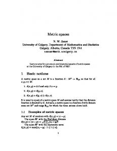
1 Introduction Object recognition and content-based image retrieval systems are highly dependent on the accurate and efficient identification of shapes. A few areas, among others, where shape analysis is of significant importance are anthropology, biology, medicine etc. For example, shapes are considered by anthropologists in building evolutionary theories or by archaeologists for dating artifacts [6]. Using images from underwater cameras, biologists study the silhouette of fish to determine seasonal migrations, as well as the health of the species, which is indicative for the quality of the water they inhabit [10]. In medicine, many diseases are identified by the pathological shape of certain cells observed from microscope images. Despite of its importance, however, shape identification is often discarded as computationally inefficient. In Figure 1: Shapes can be converted to “time series”. The this work, looking for a more optimal recognition pro- distance from every point on the profile to the center is measured and treated as the Y-axis of the time series

Here, we show that one can use some of the more accurate representations, e.g. obtain a feature vector (time series) from all shape boundary points as in Figure 1, and still construct a highly efficient matching algorithm. A key point in the proposed technique is that provided certain (reasonable) conditions are met, a rotation invariant distance between the feature vectors defines a metric over the feature space. This observation suggests that a simple, yet highly efficient pruning criterion is applicable. Namely, the triangle inequality. 2 Rotation Invariant Matching We begin by formally defining the rotation invariant matching problem. Let Ω = {Ci } be the space of all time series of length n (i.e. Ci = (c1 , c2 , . . . , cn )), extracted from shapes with an arbitrary method1 . The shape matching problem searches for the most similar b⊂Ω element to a given query Q ∈ Ω within a subset Ω b of m time series (i.e. Ω = {C1 , C2 , . . . , Cm }). As we are interested in large data collections, usually we have m  n. The similarity between Q and an arbitrary time b is measured in terms of a preselected series Ci ∈ Ω distance function d(Q, Ci ) (e.g. the Euclidean distance), defined over the entire space Ω. If the time series are aligned correctly, then the distance function, if suitable in general, will usually provide a good measure of similarity. However, if the shapes are not rotation aligned, then the corresponding time series will be misaligned too and the distance measure might produce extremely poor results. To overcome this problem we need to hold one shape fixed, rotate the other, and record the minimum distance to all possible rotations. In terms of the selected representation, every continuous rotation of a shape can be approximated by a circular shift of its vector Ci , where a circular shift is defined as Cij = (cj , cj+1 , . . . , c1 , c2 , . . .). We further denote with Ci the n by n rotation matrix which has as rows all possible circular shifts of Ci . The rotation invariant distance (rd) can now be defined as: (2.1)

rd(Ci , Q)

=

min d(Cij , Q)

1≤j≤n

The time complexity for computing the most similar shape to the query using the above rotational distance is O(mnk), where O(k) is the complexity of computing the distance function d. For example, if d is any of the Lp -norms, the complexity of the nearest neighbor search using rd as distance measure becomes O(mn2 ). When online processing of large number of queries is required 1 The

presented approach uses, but is not limited to, a centroid based-contour representation [2] (see Figure 1). Other time series representations are discussed for example in [4] and [9].

or when the data set is very large, this running time is simply untenable. 3 Best-Match Shape Searching As pointed out, searching for the most similar shape b can easily become to a given query in the data set Ω intractable as its size increases. Here we demonstrate a simple property of the rotation invariant distance that allows one to perform highly efficient best-match searches, regardless of the size of the data set. Namely, that the rotation invariant distance rd(Ci , Q) defines a pseudo-metric over the space Ω. 3.1 Metric Properties Of The Rotation Distance The distance function d(Ci , Cj ) is said to be a metric over the space Ω, if for arbitrary elements Ci , Cj , Ck ∈ Ω it satisfies the following three properties: - Positivity: d(Ci , Cj ) ≥ 0, with equality iff Ci = Cj - Symmetry: d(Ci , Cj ) = d(Cj , Ci ) - Triangle inequality: d(Ci , Cj )+d(Ck , Cj )≥d(Ci , Ck ) When only the second and the third of the above properties are satisfied, d(Ci , Cj ) is said to define a pseudometric. Showing that a distance function satisfies the triangle inequality is of particular importance when working with large data sets, as it can significantly decrease the searching time by excluding from consideration many of the data set elements. A number of techniques that utilize the triangle inequality have been proposed over the years, e.g. [1, 3], as well as some popular indexing structures as the Vantage Point trees [11]. Here we show that, provided the inner distance satisfies the triangle inequality, the rotation distance satisfies it too. Proposition 3.1. If the inner distance d(Ci , Cj ) is a pseudo-metric over the space of the shape time series Ω, then the rotation invariant distance rd(Ci , Cj ) also defines a pseudo-metric over Ω. Proof. Without loss of generality, assume that Cir0 is the rotation of Ci that has a minimal inner distance to Cj , i.e. rd(Ci , Cj ) = d(Cir0 , Cj ). Similarly, let rd(Ck , Cj ) = d(Ckr1 , Cj ) and rd(Ci , Ck ) = d(Cir2 , Ck ). Symmetry: We first note that the alignment (Cir0 , Cj ), where the first time series is rotated, corresponds to an alignment (Ci , Cjx ), where the second time series is rotated. And as d is symmetric we have rd(Ci , Cj ) = d(Cir0 , Cj ) = d(Ci , Cjx ) = d(Cjx , Ci ). This, together with definition 2.1, implies rd(Cj , Ci ) ≤ d(Cjx , Ci ) = rd(Ci , Cj ). Analogously, we can show that rd(Ci , Cj ) ≤ rd(Cj , Ci ). Hence, rd(Ci , Cj ) = rd(Cj , Ci ).

Triangle inequality: The following holds: rd(Ci , Cj ) + rd(Ck , Cj ) = d(Cir0 , Cj ) + d(Ckr1 , Cj ) ≥ d(Cir0 , Ckr1 ) ≥ d(Cir2 , Ck ) = rd(Ci , Ck ) The first inequality above is true as d satisfies the triangle inequality, and the second one follows from the fact that d(Cir2 , Ck ) is the distance between the optimal alignment of Ci and Ck , while (Cir0 , Ckr1 ) also corresponds to an alignment between the same time series. 3.2 Efficient Best-Match Searching This section introduces a scheme for fast rotation invariant bestb The speed-up in the match searching in the subspace Ω. scheme results from several levels of pruning different distance computations: 1. Pruning of rotation distance computations. The previously derived property allows us to avoid computing a large percentage of the rd distances between the query Q and the elements of the data b set Ω. 2. Pruning of inner distance computations. As the inner distance d also satisfies the triangle inequality, for every time series Ci that was not pruned on the previous level, only part of the inner distances between Q and the rotated versions of Ci need to be computed.

Algorithm 1 Rotation invariant best-match search Preprocessing: b - preselected center 1: Cr ∈ Ω 2: RL = {rd(Cr , Ci )} - sorted list, i ∈ [1..m] j 3: DLi = {d(Ci1 , Ci )} - sorted lists, i ∈ [1..m], j ∈ [1..n] Search: b Cr , RL, rd) 4: ∀Q: [bm Q, M in Dist] = RI Search(Ω, procedure [bm, ξ]=RI Search(Cnd, C, L, df ) in: Cnd: candidates; C: center; L: list of distances; df : distance function

out: bm: best-match; ξ: minimal distance 5: ξ = df (C, Q) 6: bm = C 7: Cnd = Cnd \ C 8: while Cnd 6= ∅ do 9: using the sorted L, select Ci ∈ Cnd such that: |df (Ci , C) − df (Q, C)| ≤ |df (Cj , C) − df (Q, C)|, ∀Cj ∈ Cnd, i 6= j 10: if df = rd then 11: [bmf ake , ξtmp ] = RI Search(Ci , Ci1 , DLi , d) 12: else 13: ξtmp = EarlyAbandon(Ci , Q, ξ) 14: end if 15: if ξtmp < ξ then 16: ξ = ξtmp bm = Ci 17: end if 18: ∀Cl ∈ Cnd ∧ |df (Cl , C) − df (Q, C)| > ξ: Cnd = Cnd \ Cl 19: end while

3. Pruning of primitive distance operations. Using a simple technique, called early abandon (to be described later), one can further speed up the inner distance computations that were not pruned in the previous step, by skipping some of the primitive also precompute the self-distances between Ci and its pairwise computations between the scalar elements rotations and store them in1 a jsorted n-dimensional vector DLi , i.e. DLi = {d(Ci , Ci )}, ∀j ∈ [1..n] (Note of the compared time series. that we do not store the n by n Ci matrices, but just All three levels contribute to the speed-up of the nearest the distance vectors). Maintaining all m self-distance neighbor searches in the rotation invariant space, but it vectors is necessary for the second level inner distances is the pruning of rotation distance computations that pruning and increases twice the memory requirement becomes of particular importance especially as the data for the proposed scheme compared to the simple brute set size grows very large. It is important to note that, as force search. This linear increase in space complexity a pruning criterion is applied only when the distance to is a reasonable and acceptable overhead, as it refers an element is guaranteed to be larger than some already to the compact 1D time series representation rather found distance, the algorithm is guaranteed to make no than the 2D original images. The pseudo-code with a false dismissals. detailed explanation of the rotation invariant searching is presented as Algorithm 1. For clarity of presentation 3.2.1 Best-Match Searching Algorithm The the described algorithm returns only the best-match to proposed scheme is an adaptation of Burkhard-Keller’s a given query and the optimal distance. An extension fast file searching algorithm described in [1]. Here we finding the k most similar time series to the query is assume that all rotation distances from the elements of straightforward. b to a preselected center point Cr (see Section 3.2.2) Ω For every incoming query the search routine are computed and stored in a sorted list RL. We RI Search is invoked with: a best-match candidates

b the list RL list Cnd initialized as the whole data set Ω; of the precomputed rotation distances from all data set elements to the center point; and the type of distance function set to rd. The distance function is also used to differentiate between the first and second levels of pruning. RI Search sets the initial best-match element bm to the center point and the current minimal distance ξ to the distance between the query and the center. The iterative search of the candidates list then proceeds in three steps. While the list is not empty, a new candidate is selected (line 9), using the heuristic suggested by Burkhard and Keller (described below). If the distance to the new candidate is smaller than the current minimal distance, then the best-match so far is updated to the new candidate (line 16). Finally, the triangle inequality is applied (line 18) to prune all candidates that are guaranteed to be further from the query than ξ. More precisely, as df = rd or d which both satisfy the triangle inequality, the following two inequalities hold: df (Q, Cl ) + df (Q, C) ≥ df (Cl , C) and df (Q, Cl ) + df (Cl , C) ≥ df (Q, C), or in a more compact form df (Q, Cl ) ≥ |df (Cl , C) − df (Q, C)|. Therefore, if the difference of the already computed df (Cl , C) and df (Q, C) is larger than the currently minimal distance ξ, then the distance from the query to the candidate Cl is guaranteed to be also larger than ξ, and there is no need to explicitly compute it. For the first step, the candidate selection, Burkhard and Keller suggest choosing an element Ci still in the candidates list, for which the difference |df (Ci , C) − df (Q, C)| is minimal (line 9). Note that this difference is a lower bound for the distance df (Q, Ci ), thus it is likely that by choosing the element with the minimal difference we are also choosing an element that is closer to the final solution. In the experimental evaluation we found out that the heuristic is essential for the pruning capability of the algorithm and its faster convergence to the solution. As the distance list L is sorted, the first candidate can be selected in logarithmic time. Suppose the binary search for a candidate shows that df (Ci , C) < df (Q, C) < df (Ci+1 , C), where i corresponds to the position of df (Ci , C) in the sorted list L. This means that the heuristic will return as candidate either Ci or Ci+1 . On subsequent iterations, one does not need to perform the binary search again but rather select the candidate that is still in the candidates list and whose distance to the center is closest to df (Q, C) in either direction left or right. When the algorithm is invoked with the rotation distance rd as distance function, i.e. we are on the first pruning level, the selected candidate Ci needs to be rotated n times and the inner distances d(Cij , Q), j ∈

[1..n] need to be computed. We can do this again by applying the RI Search procedure (line 11, second pruning level), this time with a center Ci1 , sorted list of distances to the center DLi , and the inner distance d as a distance function. The list of candidates is now composed of every rotation of Ci , which is simply the rotation matrix Ci . When a candidate Cij for an inner distance computation is identified, the actual inner distance d(Q, Cij ) can be optimized further by computing it with an early abandon technique (line 13, third pruning level). The EarlyAbandon procedure is a simple, yet extremely efficient technique for speeding up the computations of a distance function (see Section 4). It can be applied for an arbitrary Lp -norm and uses the minimal so far distance ξ. P Rather than computing the entire sum n p 1/p Lp (C, Q) = , EarlyAbandon exists i=1 (|ci − qi | ) the computation if at some point it exceeds ξ, and hence cannot improve on the currently best match. 3.2.2 Center Selection The performance of the algorithm, is highly dependent on the pruning capability of the selected center Cr . In the original BurkhardKeller algorithm, the selection is made at random. There are two factors that determine how good Cr is, b with respect to namely, its position in the subspace Ω the other data set points, and its position with respect to the queries. A suitable center point will have a small difference |rd(Cj , Cr )−rd(Q, Cr )| for just a few data set points Cj . Shapiro [8] argues that good centers can be points, which are further from the center of any cluster that might be present in the data set. This is so, because points close to the cluster centers will be in close proximity to many other points, and for most of those neighbors the above difference will be small. In our implementation, rather than randomly selecting the center, we use subsampling. For the purpose, the preprocessing step (line 1, Algorithm 1) is modified as follows. A small training and validation subsets, are b The center Cr is set to the randomly selected from Ω. point from the training subset that has the best pruning capability for the queries from the validation set. The subsampling implicitly takes into consideration the specific data distribution, which leads to better pruning ability and smaller variance as compared to random center selection. The above preprocessing is performed only for the first pruning level. For the second pruning level we always use as centers the original series, i.e. Ci1 . Still, as seen from the evaluation in Section 4, the variance in the performance is very small, which suggests that any rotation Cij is an equally suitable center. An intuition of the phenomenon is provided by the ob-

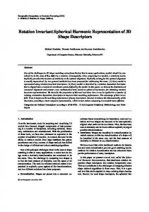
servation that for Lp -norms the following equality is (j +k)mod(n) (j +k)mod(n) ), ) = d(Cij2 , Ci 2 true: d(Cij1 , Ci 1 j1 , j2 , k ∈ [1..n]. The fact implies that every rotation Cij is distributed in the same way among the rest of the rotations of Ci . 4 Experimental Evaluation The performance of the RI Search algorithm is evaluated, utilizing the Euclidean distance as inner metric. The speed-up introduced by the presented approach is discussed for two publicly available shape data sets, each exhibiting different properties as density of the available clusters and separability between them. To illustrate the contribution of the individual pruning levels, a break-up of the improvement into components has also been provided. All experiments represent averages over 50 randomly drawn queries, that are subsequently removed from the data sets. ARROWHEADS Data Set. The data set represents a large collection of arrowheads with various shapes and sizes. Figure 2 depicts some representative classes from the data.

Figure 2: Arrowheads data set. Representative examples. We have further augmented the data set with new images by scaling, deforming and rotating some of the original shapes. The overall size of the resulting data set is 15000 samples. After extracting the time series from the shapes, we resample them to n = 250 time points, which for this data set seems to preserve the accurate representation. Prior to storing, all resampled time series have further been normalized to have a mean zero and standard deviation one. The percentage improvement of our approach over the BruteForce search in terms of performed primitive distance computations is illustrated on Figure 3, left. The performance of simply applying the EarlyAbandon technique is also included for comparison. There are several important aspects to observe in the result. Increasing the space density, i.e. introducing more samples in the data set, increases the pruning power of the algorithm. The effect is expected as with more elements the chance of finding a sample that is very close to the query is higher. Such samples mini-

Figure 3:

Arrowheads. Improvement over BruteForce search. Left: Expected percentage of primitive operations to be performed. Right: Expected running time.

mize significantly the cut-off threshold ξ, and a lot of the remaining elements start failing the triangle inequality test. For the largest data set the RI Search algorithm performs twenty times less operations than simply applying EarlyAbandon (0.19% vs 3.88% operations). For all data set sizes of 500 elements and above the RI Search algorithm performs less than 1% of the operations performed by the exhaustive BruteForce search algorithm. The time improvement does not correlate exactly to the operations improvement because of the overhead for searching the sorted candidates and distances lists. Overall, the proposed algorithm is from four (m = 32) to more than fifty (m = 15000) times faster than the BruteForce search (see Figure 3 right). It is important to understand how much each pruning component contributes for the final operations improvement introduced by the algorithm. Fewer computations of the rotation distance imply accessing fewer shapes, which is essential especially when indexing is applied. And fewer inner distances to be considered suggest less memory accesses to different elements. Table 1 gives a break-up for RI Search into levels of pruning. Table 1: Percentage of performed operations. Row1 : Percentage of computed rotation distances. Row2 : Percentage of computed distances out of all possible inner distances after level one was performed. Row3 : Percentage of primitive operations out of all possible remaining operations after level two was performed Pruning Mean(Deviation) of Performed Operations(%) Level m = 250 m = 1000 m = 15000

1-st 2-nd 3-rd

52.1(12.3) 19.9(0.85) 16.0(0.91)

34.1(10.0) 15.5(0.79) 11.4(0.38)

22.7(5.81) 9.81(0.31) 8.61(0.30)

The table illustrates how powerful the triangle inequality is, especially for larger data sets. For exam-

ple, when m = 15000 the algorithm avoids examining almost 80% of the shapes. The second and the third pruning levels are presented with respect to the possible operations after the previous pruning level has been performed. Finally, the standard deviation in the performed operations for each pruning level is also presented in the table. The small variance in the second pruning level suggests that all rotated versions of a time series Ci are equivalent in a certain sense, as the rest of the rotated series are similarly distributed around them. Therefore, as discussed in Section 3.2.2, any rotation Cij can be considered an equally suitable choice for an inner distance center. SQUID Data Set. The data set contains 1100 images of marine creatures. Figure 4 demonstrates several samples from the database.

more than six times faster than EarlyAbandon(see Figure 5, right).

5 Conclusions In this work we demonstrated that, under certain conditions, rotation invariant distance measures define a metric over the shape space, which implies that searching in this space could be highly optimized. An algorithm was presented that exploits this observation and speeds up the best-match shape searching, by avoiding a large number of distance computations. We have currently adopted the algorithm in a hierarchical and a manifold shape clustering approaches, as well as in subsequent out-of-sample classification extensions. The efficiency of the best-match searching algorithm allowed us to scale these tasks to much larger data collection. References

Figure 4: SQUID data set. Representative examples. The shapes are preprocessed as described for the Arrowheads data set. For this data set we use the original shapes without any further transformations. All extracted time series are resampled to n = 1000 time points. The higher dimensionality suggests a more sparsely populated space, which is the reason for the worse expected improvement compared to the Arrowheads data set (see Figure 5)

Figure 5: SQUID. Improvement over BruteForce search. Left: Expected percentage of primitive operations to be performed. Right: Expected running time.

Similarly to the Arrowheads data set, increasing the number of time series leads to a linear increase in the pruning capability of the RI Search algorithm. In terms of running time, for m = 1000 the algorithm is more than sixteen times faster than BruteForce and

[1] W. Burkhard and R. Keller. Some approaches to bestmatch file searching. Commun. ACM, 16(4):230–236, 1973. [2] C. Chang, S. Hwang, and D. Buehrer. A shape recognition scheme based on relative distances of feature points from the centroid. Pattern Recognition, 24(11):1053– 1063, 1991. [3] K. Fukunaga and P. Narendra. A branch-and-bound algorithm for computing k-nearest neighbors. IEEE Trans. Comp., 24(7):750–753, 1975. [4] B. Kartikeyan and A. Sarkar. Shape description by time series. IEEE Trans. Pattern Anal. Mach. Intell., 11(9):977–984, 1989. [5] D. Li and S. Simske. Shape retrieval based on distance ratio distribution. HP Tech Report. HPL-2002-251, 2002. [6] M. O’Brien and R. Lyman. Resolving phylogeny: Evolutionary archaeology’s fundamental issue. Essential Tensions in Archaeological Method and Theory, pages 115–125, 2003. [7] R. Osada, T. Funkhouser, B. Chazelle, and D. Dobkin. Shape distributions. ACM Transactions on Graphics, 21(4):807–832, 2002. [8] M. Shapiro. The choice of reference points in bestmatch file searching. Commun. ACM, 20(5):339–343, 1977. [9] S. Tabbone, L. Wendling, and J.-P. Salmon. A new shape descriptor defined on the Radon transform. Comput. Vis. Image Underst., 102(1):42–51, 2006. [10] K. Ueno, X. Xi, E. Keogh, and D. Lee. Anytime classification using the nearest neighbor algorithm with applications to stream mining. IEEE International Conference on Data Mining (ICDM), 2006. [11] P. Yianilos. Data structures and algorithms for nearest neighbor search in general metric spaces. In 4th annual ACM-SIAM Symposium on Discrete algorithms (SODA), pages 311–321, 1993.