Fast calculation method for computer-generated ... - OSA Publishing

Fast calculation method for computer-generated cylindrical hologram based on wave propagation in spectral domain Boaz Jessie Jackin and Toyohiko Yatagai∗ Center for Optics Research and Education, Utsunomiya University, Utsunomiya 320-0072, Japan ∗ [email protected]

Abstract: A fast calculation method for computer generation of cylindrical holograms is proposed. The calculation method is based on wave propagation in spectral domain and in cylindrical co-ordinates, which is otherwise similar to the angular spectrum of plane waves in cartesian co-ordinates. The calculation requires only two FFT operations and hence is much faster. The theoretical background of the calculation method, sampling conditions and simulation results are presented. The generated cylindrical hologram has been tested for reconstruction in different view angles and also in plane surfaces. © 2010 Optical Society of America OCIS codes: (090.1760) Computer holography; (090.2870) Holographic display; (050.1960) Diffraction theory.

References and links 1. Tung H. Jeong, “Cylindrical holography and some proposed applications,” J. Opt. Soc. Am. 57, 31396–1398 (1967), http://www.opticsinfobase.org/josa/abstract.cfm?URI=josa-57-11-1396. 2. O. D. D. Soares and J. C. A. Fernandes, “Cylindrical hologram of 360o field of view,” Appl. Opt. 21, 3194–3196 (1982), http://www.opticsinfobase.org/abstract.cfm?URI=ao-21-17-3194. 3. A. W. Lohmann and D. P. Paris, “Binary Fraunhofer holograms, generated by computer,” Appl. Opt. 6, 739–1748 (1967), http://www.opticsinfobase.org/ao/abstract.cfm?URI=ao-6-10-1739. 4. J. W. Goodman, Introduction to Fourier Optics (McGraw-Hill, 1968). 5. T. Tommasi and B. Bianco, “Computer-generated holograms of tilted planes by a spatial frequency approach,” J. Opt. Soc. Am. A 10, 299–305 (1993), http://www.opticsinfobase.org/josaa/abstract.cfm?URI=josaa-10-2-299. 6. Y. Sakamoto and M. Tobise, “Computer generated cylindrical hologram,” in Practical Holography XIX: Materials and Applications, Tung H. Jeong and Hans I. Bjelkhagen, eds., Proc.SPIE 5742, 267–274 (2005). 7. A. Kashiwagi and Y. Sakamoto, “A Fast calculation method of cylindrical computer-generated holograms which perform image reconstruction of volume data,” in Adaptive Optics: Analysis and Methods/Computational Optical Sensing and Imaging/Information Photonics/Signal Recovery and Synthesis Topical Meetings on CD-ROM, OSA Technical Digest (CD) (Optical Society of America, 2007), paper DWB7, http://www.opticsinfobase.org/abstract.cfm?URI=DH-2007-DWB7. 8. T. Yamaguchi, T. Fujii, and H. Yoshikawa, “Fast calculation method for computer-generated cylindrical holograms,” Appl. Opt. 47, D63–D70 (2008), http://www.opticsinfobase.org/ao/abstract.cfm?URI=ao-47-19-D63. 9. T. Yamaguchi, T. Fujii, and H. Yoshikawa, “Computer-generated cylindrical rainbow hologram,” in Practical Holography XXII: Materials and Applications, Hans I. Bjelkhagen and Raymond K. Kostuk, eds., Proc.SPIE 6912, 69121C (2009). 10. Y. Sando, M. Itoh, and T. Yatagai, “Fast calculation method for cylindrical computer-generated holograms,” Appl. Opt. 13, 1418–1423 (2005), http://www.opticsinfobase.org/oe/abstract.cfm?URI=oe-13-5-1418. 11. G. E. Williams, Fourier Acoustics, Sound Radiation, and Near-field Acoustical Holography (Academic Press, 1999).

#134731 - $15.00 USD

(C) 2010 OSA

Received 8 Sep 2010; revised 11 Oct 2010; accepted 17 Oct 2010; published 22 Nov 2010

6 December 2010 / Vol. 18, No. 25 / OPTICS EXPRESS 25546

12. N. N. Lebedev, Special Functions and Their Applications (Prentice Hall, 1965), pp. 98–160. 13. G. B. Arfken and H. J. Weber, Mathematical Methods for Physicists (Academic Press, 2001), pp. 702–705.

1.

Introduction

Holograms can record and reproduce all the three dimensional informations like motion parallax, accommodation, occlusion, convergence and so on. Hence it is possible to perceive a threedimensional object very close to reality, when looking into a hologram, from any direction. But the potential of the holography is restricted by the geometrical shape of the hologram. Usually holograms were made of flat surfaces, which has a limited viewing angle. This constraint can be overcome if holograms were made on cylindrical surfaces. A cylindrical hologram has a “look around proerty” and hence can be observed from any direction [1] [2]. In other words, by making a computer generated cylindrical hologram, we would have virtually created an object that never existed. Cylindrical geomerty has also proved to be very efficient in 3D volumetric imaging such as in Magnetic Resonance Imaging and Computed Tomography. Due to these appealing facts more interest has been generated in computer generated cylindrical holography in the recent years. Inorder to appreciate the usefulness and challenges in this, a very short review of the evolution of computer generated cylindrical holography is presented below. In early days holograms were made for real existing objects using lasers. Then with the development of computers, the method was extended to non existing objects in the form of computer generated holography [3]. In this process the optical recording setup is simulated and the generated pattern in transfered into a photographic film. The scalar diffraction theories which defines the wave propagation were at the heart of this simulation process [4]. These theories were able to use FFT algorithm for computation and hence holograms were generated with reasonable speed. But FFT can be used only if the object and hologram surface holds a shift invariance relationship. Hence computer generated holograms were usually made for geometries where the object and hologram sufraces are planar and perpendicular to the optical axis. Later on the method was improved and fast computation schemes using FFT were also developed for non shift invariant systems such as, a tilted plane geometry [5]. But for a long time the cylindrical geometry was not considered for making a computer generated hologram. The main reason was the extreme difficulty in devicing a fast computation method for a curved hologram surface. But the recent developments in technology and the possibility of producing advanced display and recording devices, has made people focus on cylindrical geometries. As a result, papers describing cylidrical computer generated holography started to appear in the recent five years. Y.Sakamoto et al [6] used the angular spectrum of plane waves method to generate a cylindrical hologram of a plane object. They employed the shift invariance in rotation between a planar and cylindrical surface and hence could use FFT. Then they imporved on their method to generate the hologram of a volume object by slicing it into planar segments [7]. This took 2.76 hrs to calculate the hologram of a 13×13×13 mm object. Yamaguchi et al [8] used the Fresnel transform and segmentation approach to generate cylindrical holograms. Since they did not use FFT, the computation time was 81 hrs on a parallel computing machine for an object of size 15×15×15 mm. They also developed a computer generated cylindrical rainbow hologram using the same method [9]. The calculation time for the rainbow hologram was 45 min on a single computer, but sacrifices vertical parallax. Sando et.al [10] generated cylindrical holograms by defining propagation in spatial domain using convolution. In this method the shift invariance was preserved by choosing the object also to be a concentric cylindrical surface with the hologram. Hence FFT could be used and they had used three FFT loops for simulating wave propagation. So far no one has computed a cylindrical hologram by considering wave propagation from a cylindrical surface in spectral domain. This paper proposes to do the same using

#134731 - $15.00 USD

(C) 2010 OSA



a spectral method in cylindrical coordinates . In other words, this method is the counter part of angular spectrum of plane waves in cartesian coordinates. This method uses only two FFT calculations, for simulating wave propagation and hence more faster. But the difficulty lies in finding the transfer function analytically, which is the heart of this computation procedure. Section 2 explains the theoretical background of the computation method and the derivation of Transfer Function, starting from the wave equation. The computation procedure with sampling conditions are explained in Section 3. Two reconstruction schemes to test the correctness of the hologram is presented in Section 4. A discussion on the results and concluding remarks are presented in Section 5. 2.

Theoretical background

An electromagnetic field is defined by Maxwells equations and its propagation by the Helmholtz equation. Hence to find the complex amplitude of a propagating wave at any instance of time and any where in space, the solution to the Helmholtz equation is required. The Helmholtz equation in p is given by ¡ 2 ¢ ∇ + k p = 0, (1) where k is the wave number, given by k = 2π /λ , and p denotes the complex amplitude of the wavefront as a function of spatial coordintes. The solution to the Helmholtz equation in cylindrical co-ordinates, as shown in Fig. 1 can be represented as shown in Eq. (2) p(r, φ , y) = R(r)Φ(φ )Y (y),

(2)

where R(r),Φ(φ ) and Y (y) represent the radial, angular and vertical components, respectively On solving by separation of variables, (1)

(2)

R(r) = R1 Hn (kr r) + R2 Hn (kr r), (1)

(2a)

(2)

where Hn and Hn are the Hankel functions of first and second kind, respectively. Φ(φ ) = φ1 einφ + φ2 e−inφ ,

(2b)

Y (y) = Y1 eiky y +Y2 e−iky y ,

(2c)

Hence the most general solution to Eq. (1) according to Eq. (2a) - (2c) in the spectral domain is given by ∞

p(r, φ , y) =

∑

n=−∞

einφ

1 2π

Z∞ h

i (2) (1) An (ky )eiky y Hn (kr r) + Bn (ky )eiky y Hn (kr r) dky ,

(3)

−∞

where An (ky ) and Bn (ky ) are the arbitrary constants. We now consider a special case according to the following assumptions. 1. Let all the radiating sources be within the circular cylinder of radius ‘a’, i.e, the radiating source is cylindrical surface of radius ‘a’ 2. The complex amplitude is measured only at positions outside the cylindrical radius ‘a’ ie, we consider only outward propagation. Let the measuring position be denoted by ‘r’.

#134731 - $15.00 USD

(C) 2010 OSA



Fig. 1. Coordinate system.

Applying these assumptions to Eq. (3), it reduces to, ∞

∑

p(a, φ , y) =

e

1 2π

inφ

n=−∞

Z∞

(1)

An (ky )eiky y Hn (kr a)dky ,

(4)

−∞

for which a detailed explanation can be found in [11] Now, let us consider Pn (r, ky ) to be the two-dimensional Fourier transform in φ and y in cylindrical coordinates Pn (r, ky ) ≡

1 2π

Z2π

Z∞

p(r, φ , y)e−inφ e−iky y dy,

dφ

(5)

−∞

0

The inverse relation for Eq. (5) is given by ∞

∑

p(r, φ , y) =

e

inφ

n=−∞

1 2π

Z∞

Pn (r.ky )eiky y dky ,

(6)

−∞

where n can take only integer values because the cylindrical surface is a closed one in the circumferential direction. Comparing Eq. (6) at r = a with Eq. (4) we get (1)

Pn (a, ky ) = An (ky )Hn (kr a),

(7)

Using Eq. (7) to eliminate An in Eq. (4) yields ∞

p(r, φ , y) =

∑

einφ

n=−∞

1 2π

Z∞

(1)

Pn (a, ky )eiky y −∞

Hn (kr r) (1)

Hn (kr a)

dky ,

(8)

Eq. (8) calculates the complex amplitude at any position p(r, φ , y), for ((r > a)), when the complex amplitude in a cylindrical surface of radius ‘a’ is given. The spectral soulution in Eq. (8) is similar in form to the angular spectrum of plane waves which is defined as p(x, y, z) =

#134731 - $15.00 USD

(C) 2010 OSA

1 4π 2

Z∞

Z∞

dkx −∞

dky P(kx , ky , z0 )ei(kx x+ky y) eikz (z−z0 ) .

(9)

−∞



For an easy understanding, the spectral solution in cylindrical coordinates (Eq. (8)) can be compared with the spectral solution in cartesian coordinates (Eq. (9)). On comparison one could understand that (a) The spectral component in Eq. (8) can be represented as shown in Eq. (10) 1 Pn (a, ky ) = 2π

Z2π

Z∞

p(a, φ , y)e−inφ e−iky y dy,

dφ 0

(10)

−∞

which is nothing but a Fourier transform realation. We would like to follow the convention mentioned by Earl.G.Williams [11] and call this spectrum as the Helical wave spectrum. (b) The propagation component in Eq. (8) (Transfer function) is given by (1)

T (a, ka , r, kr ) = q where kr =

k2 − ky2

and

Hn (kr r) (1)

Hn (kr a)

,

(11)

k = 2π /λ .

When ‘r’ in Eq. (8) is kept constant, ie, the measurement plane (hologram surface) is also a cylinder, then the system is shift invariant. Hence we can use FFT to evaluate Eq. (8) and hence fast calculation. Deriving out the analytical expression for the Transfer Function for propagation from cylindrical surface as shown in Eq. (11), is the most important step in this work. For a detailed understanding and more insight into the theory explained above, the reader may refer to [12] [13]. 3.

Computational Procedure

The schematic and geometry of the simulation problem are shown in Fig. 2. The object and hologram are concentric cylindrical surfaces with radius a and r respectively. The height of the cylindrical surfaces were y = h. The object of size N × N was chosen for simulation which is graphically represented in Fig. 3. The object is illuminated virtually by a point source form the center which also serves as the reference. 3.1.

Sampling Conditions

Now, inorder to achieve proper reconstruction, the Nyquist sampling conditions must be satisfied. For this the discrete transfer function’s rate of change should be less than or equal to π when n = N/2, where N = [−N/2...0...N/2]. From the analysis of Eq. (11) the spatial rate of change of kr r is higher than that of kr a. Hence as long as the sampling condition for kr r is satisfied, the entire Transfer function also meets the sampling condition approximately. Accordingly the Nyquist sampling condition can be expressed by the inequality as shown in below ¯ q ¯ ¯ ∂ ¯¯ 2 kr 1 − (λ ky ) ¯¯ ≤ π, (12) ¯ ∂n n=N/2 from the above inequality with conditions, ky = n∆ky ,∆ky = ∆L1 0 and k = the height of the cylinder) we can obtain ¯ ¯ ¯ ¯ ¯ ¯ 2 ¯ ¯ kλ rn ¯ ¯ r ≤ π, ¯ ¯ ¯ ∆L2 1 − λ 2 n2 ¯ 2 ¯ ¯ 0 ∆L 0

#134731 - $15.00 USD

(C) 2010 OSA

2π λ ,

(where ∆L0 = h is

(13)

n=N/2



Fig. 2. Recording setup: (a) schematic and (b) geometry.

which again reduces to

s 2nrλ ≤ ∆L0

as ∆L02 À λ 2

¡ N ¢2 2

∆L02 − λ 2

µ ¶2 N , 2

(14)

and is usually satisfied, a better approximation of the above inequality is √ Nrλ

∆L02 . (15) rλ Based on the sampling condition, the dimensions for the simulation problem were choosen. Accordingly, the object and hologram were assumed to be cylindrical surfaces with radius a = 1cm and r = 10cm respectively. The height of the cylindrical sufrace was assumed to be y = 10cm. To avoid harsh sampling requirements, the wavelength λ was assumed to be large i.e, λ = 180µ m. When all these dimensions were substituted in the sampling condition, given by Eq. (15), the required number of samples turned out to be N ' 512. Hence the object and transfer functinon were generated as 512×512 matrices. ∆L0 ≥

(or)

N≥

3.2. Hologram generation The computation procedure to generate the hologram can be summarized as follows 1. The transfer function(TF) was generated according to Eq. (11). 2. The complex amplitudes of object and reference were generated as 512 × 512 matrices. The generated object is graphically shown in Fig. 3 3. The Fourier spectrum of object and reference wavefield was computed (using FFT) according to Eq. (5) which gives the corresponding complex amplitude in spectral domain at the object surface. 4. The calculated spectrum (object and reference) is multiplied with the transfer function which gives the corresponding complex amplitude in spectral domain at the hologram surface.

#134731 - $15.00 USD

(C) 2010 OSA



5. The complex amplitude in spectral domain is inverse Fourier transformed according to Eq. (6) to get the complex amplitude in real space at the hologram surface 6. The complex amplitudes due to object and reference are added(superposed) at the hologram surface and their intensity is calculated.

Fig. 3. Object.

Fig. 4. Hologram.

The numerical computation of the above said procedure can be expressed as shown below Hologram = |IFFT [FFT (Ob ject) × T F] + IFFT [FFT (Re f erence) × T F]|2 where, Hologram is the resulting 2D image(matrix) that holds the intensity pattern of hologram, T F is the transfer function and FFT and IFFT are the forward and inverse discrete fast Fourier transforms respectively. The calculated intensity pattern is the hologram and is graphically shown in Fig. 4 3.3.

Simulated reconstruction

The same numerical method that was used for generating hologram, is used to reconstruct the hologram. The hologram is reconstructed on the original cylindrical surface (object surface). Inorder to achieve this, the reconstruction is simulated such that the conjugate of the reference is used to illuminate the hologram. The numerical computation of the reconstruction can be expressed as follows, Reconstruction = |IFFT [FFT (Hologram ×Con jugate[Re f erence]) × T F]|2 where, Reconstruction is the 2D image(matrix) that holds the reconstructed intensity distribution, T F is the transfer function and FFT and IFFT are the forward and inverse discrete fast Fourier transforms respectively. The reconstructed image pattern is shown in Fig. 5 which exactly resembles the original object choosen. 4.

Testing the hologram

The hologram generated using this method is tested for correctness and other reconstruction capabilities. Three reconstruction schemes were used, and are explained below. 4.1.

Reconstruction in plane surface

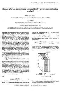
The reconstruction of the cylindrical object on plane surfaces, defined at distances z = 1 and z = −1 is simulated. The schematic and geometry of this setup are shown in Fig. 6. The width

#134731 - $15.00 USD

(C) 2010 OSA



Fig. 5. Reconstruction-Cylindrical surface.

Fig. 6. Planar reconstruction: (a) schematic and (b) geometry.

and height of the reconstruction plane were set to be 3 cm and 10cm respectively. Each reconstruction plane coincides with the original cylindrical object only at one position, ie at θ = 0◦ and at θ = 180◦ . Hence during reconstruction, only these two vicinities(of the object) are expected to be reconstructed in focus and other areas unfocused. But now, these two reconstruction planes nomore maintain any shift invariance relation to the hologram surface and hence FFT cannot be used for reconstruction. Hence the reconstruction was done using direct integration according to Eq. (16) shown below ZZ

U(a, φ , z) =

U(r, θ , z)exp(ikr) dφ dz. r

(16)

The reconstructed images for planes z = 1 and z = −1 are shown in Fig. 7 and Fig. 8 respectively. As seen from the Fig. 7 only the letter ‘P’ that lies in the vicinity of θ = 0◦ is in focus. While Fig. 8 shows the letter ‘O’ which is in the vicinity of θ = 180◦ reconstruced sharply. Hence the cylindrical hologram could reconstruct the stored data properly in any surface.

#134731 - $15.00 USD

(C) 2010 OSA



Fig. 7. Planar Reconstruction (z=1).

4.2.

Fig. 8. Planar Reconstruction (z=-1).

Reconstruction for variable viewing angles

The hologram was also reconstructed for viewing from a particular direction for a particular viewing angle, on the cylindrical surface as shown in Fig. 9.

Fig. 9. Variable angle reconstruction - Schematic.

Fig. 10. 120◦ (−60◦ to 60◦ ) view angle.

Fig. 11. 90◦ (90◦ to 180◦ ) view angle.

Fig. 12. 45◦ (−180◦ to −135◦ ) view angle.

Here three cases were considered, one for a viewing angle of 120◦ ie.(−60◦ to 60◦ ) and another for 90◦ (90◦ to 180◦ ) and the other for 45◦ (−180◦ to −135◦ ). The direct integration formula, shown in Eq. (16) was used to simulate reconstruction. The reconstructed results for viewing angle −60◦ to 60◦ , 90◦ to 180◦ and −180◦ to −135◦ are shown in Fig. 10, Fig. 11

#134731 - $15.00 USD

(C) 2010 OSA



and Fig. 12 respectively. The letters ‘APA’ that fall in the vicinity of −60◦ to 60◦ are alone reconstructed in Fig. 10. While the letter ‘C’ and half of the letter ‘O’, that fall in the vicinity of −180◦ to −90◦ are reconstructed in Fig. 11. Similarily the view angle of 45◦ reconstructs only half of the letter ‘O’ and half of ‘R’ that lie within −180◦ to −135◦ as shown in Fig. 12. Hence the hologram was able to reconstruct the stored information properly. 5.

Concluding Remarks

A fast calculation method for computer generation of cylindrical holograms based on wave propagation from cylindrical surfaces in spectral domain, is proposed. It uses only two FFT calculations for simulating wave propagation and hence is believed to be the fastest among existing methods for cylindrical CGH. The holograms were able to reconstruct the images very precisely. Simulated reconstruction in planar surfaces and for variable viewing angles also produced correct results. Table 1. Calculation time

Task

Time(seconds)

Load Object

0.018

Generation of Transfer Function

6.36

Calculation of reference wavefont at hologram plane

0.054

Calculation of object wavefont at hologram plane

0.15

Calculation of hologram (interference)

0.095

The calculation time for this computation method using sample size of 512 × 512 on a 2.7 GHz CPU is shown in Table. 1. It takes a total of 6.67 seconds for the entire calculation. As seen from the table, generation of the Transfer function consumes the maximum time. The next most time consuming operation is the simulation of the object wavefont at the hologram plane. This operation includes two FFT loops and the time consumed increases nonlinearly with increase in number of samples. While the time consumed by the generation of transfer function operation increases only linearly. Simulation in optical wavelengths demands atleast 30, 000 × 30, 000 sampling points for an object of diameter 10 cm to give satisfactory results. Hence it is the FFT operation that will consume the maximum time on an ordinary computer when calculating in optical wavelengths. But a GPU computing system can dramatically increase the speed of FFT, especially for very large sampling points. The generation of transfer function also includes only simple arithmatic and is easily paralleizable and hence can be generated very fast using a GPU. Hence this calculation method which is highly parallelizable and uses only two FFT’s, should be able to generate holograms in real time for optical wavelengths. The two main bottle necks in the field of computer generated holography and digital holography are i) computation speed and ii) resolution of recording and display devices. This, along with the unavailability of cylindrical shaped recording and display devices, is the main constraint in realising the proposed method. But with the sudden development in nanotechnology, we are not far from the days to have recording and display devices with pixel pitch in the order of hundreds of nanometers. It may also be possible to produce them in cylindrical or any other shape. Then the other constraint, which is computation speed, can be improved by implementing, a) new fast calculation methods and b) parallel processing using GPU. Hence we believe, this work which is a new and fast calculation method will be a small step towards realising realtime recording and reconstruction of digital cylindrical holograms.

#134731 - $15.00 USD

(C) 2010 OSA

