Oc Physica-Verlag/Springer 2004. FAST CROSS-VALIDATION IN ROBUST. PCA. Sanne Engelen and Mia Hubert. Key words: Cross-validation, robustness, fast ...
COMPSTAT’2004 Symposium
c Physica-Verlag/Springer 2004 �
FAST CROSS-VALIDATION IN ROBUST PCA Sanne Engelen and Mia Hubert Key words: Cross-validation, robustness, fast algorithm. COMPSTAT 2004 section: Partial least squares. Abstract: One of the main issues in Principal Component Analysis (PCA) is the selection of the number of principal components. To determine this number, the Predicted Residual Error Sum of Squares (PRESS) value is frequently used [2], [8]. It can be computed on a validation set, but such a new data set is not always available and many data sets in chemometrics or bioinformatics have a too small size to split into a training set and a validation set. Therefore, a cross-validated version of the PRESS statistic can be used, which is obtained by removing one observation at a time from the total data set. This technique is however rather time consuming. The computational complexity increases even more when robust PCA methods are used, such as the MCD estimator [12] for low-dimensional data or the ROBPCA method [4] for high-dimensional data. In this paper we introduce faster algorithms to compute the cross-validated PRESS value for these two methods. We evaluate the developed procedures by means of simulated and real data in both low and high dimensions. We also extent the methodology to high-breakdown regression methods such as the LTS estimator [15], MCD-regression [13], robust principal component regression [7] and robust PLS regression [6].
1
Introduction
The comparison of different estimators is a very important issue in statistics. One possibility is to compare them based on their predictive ability. For this purpose the Predicted Residual Error Sum of Squares (PRESS) is very well suited (see e.g. [1] and [11]). In general it is defined as the sum of the squared residuals from a validation set. The model parameters on the other hand are estimated from an independent training set. However, a validation (or test) set is not always available and many data sets in chemometrics or bioinformatics have a too small size to split into a training set and a validation set. Therefore, a cross-validated version of the PRESS statistic can be used. To compute the residual of case i, this observation is first removed from the data set before the parameters are estimated. This one-fold cross-validation is very popular, but is very time consuming. Only in very specific cases, like linear regression, the cross-validated residuals can be calculated using closed formulas. Therefore one-fold cross-validation is usually applied to smaller data sets. Note that at larger data sets, m-fold cross validation is a valuable alternative.
990
Sanne Engelen and Mia Hubert
In this paper we concentrate on two robust PCA methods: the MCD estimator [12] for low-dimensional data and the ROBPCA method [4] for high-dimensional data. Contrary to classical PCA, they are resistant to outliers in the data. Although their computation time is reasonable (e.g. it takes 4.16 seconds to run ROBPCA on a data set with n = 180 observations in p = 750 dimensions on a Pentium IV with 2.4 GHz), it is no longer feasible to execute the full algorithm n times. Fast cross-validation is thus certainly needed for these robust methods. In the next section, we first define a robust cross-validated PRESS value. In Section 3 we introduce fast algorithms for its computation. In Section 4 and 5 we illustrate the performance of our method by means of simulations and examples. Matrices will be denoted by capital letters. Our data matrix Xn,p has n observations and p dimensions. A vector is always indicated with a bold symbol e.g. xi = (xi1 , · · · , xip )� stands for the ith observation.
2
A robust PRESS value
PCA [8] is a well-known dimension reduction technique where a k-dimensional loading matrix Pp,k and scores ti are constructed such that � ˆ (xi − µ) ti = Pk,p
(1)
ˆ an estimate of the center of the data. In classical PCA, µ ˆ is given with µ by the mean of the data and the k loading vectors are the eigenvectors of the empirical covariance matrix of the data that belong to the k largest ˆ and P for robust PCA methods eigenvalues. Details of the construction of µ are given in Section 3 for the MCD-algorithm and in reference [4] for the ROBPCA method. An estimate of xi in the k-dimensional PCA-space is given by ˆ ˆ i,k = Pp,k ti + µ. (2) x The cross-validated PRESSk value is then defined as PRESSk =
n
ˆ −i,k 2
xi − x
(3)
i=1
ˆ −i,k the estimate of the ith observation based on a PCA model with with x k components constructed from the n − 1 other samples. ˆ −i,k in (3) are based on a robust PCA method, Even if the fitted values x the PRESS value is not robust as it also includes the prediction error of the possible outliers. A robust version of the PRESS is obtained by adding weights to each observation: R-PRESSk =
n i=1
ˆ −i,k 2 . wi xi − x
(4)
Fast cross-validation in robust PCA
991
These weights wi are determined before the cross-validation is started. Based on the PCA estimates on the full data set for k = 1, . . . , kmax components, outliers for every model under investigation are marked. For details about the definition of an outlier in PCA, we refer again to [4]. If an observation is an outlier in one or more models, its weight wi equals 0. Samples that are never detected as an outlier, obtain weight wi = 1. Doing so, the robust PRESSk value is based on the same set of observations for each k. This definition is similar to the robust RMSECV value that is defined for robust PCR [7] and robust PLS regression [6].
3
Fast cross-validation
The MCD (Minimum Covariance Determinant) estimator [12] is a highly robust method to estimate multivariate location and scatter parameters when the number of variables p is smaller than half the number of samples n. The principal components can be considered as the eigenvectors of the robust covariance estimate. ROBPCA [4], ROBust Principal Components Analysis, on the other hand is a technique where projection pursuit ideas are combined with the MCD estimator and is in particular appropriate for high-dimensional data. In order to explain how the calculation of the PRESS values can be speeded up for MCD, we first describe the original FAST-MCD algorithm [14]. Then we present the adapted version and indicate where some time improvements of the original procedure are made. For a detailed description of the ROBPCA algorithm and its changes towards fast cross-validation (which are comparable with those of MCD), we refer to [4] and [3]. Here, we will only show the numerical results.
3.1
The MCD estimator
The objective of the raw MCD is to find h > n2 observations out of n whose covariance matrix has the smallest determinant. Its breakdown value is [n−h+1] , n hence the number h determines the robustness of the estimator. For its computation, the FAST-MCD algorithm [14] can be used. It roughly proceeds as follows : 1. Many random (p + 1)-subsets are drawn, which are enlarged to initial h-subsets using a C-step as explained in the next step. If it is computationally feasible, all possible (p + 1)-subsets are used. Else 500 (p + 1)-subsets are drawn. 2. Within each h-subset, two C-steps are performed. Basically a C-step ˆ 0 and the classical coconsists of computing first the classical center µ ˆ 0 of the h observations. Then the robust distance variance matrix Σ
992
Sanne Engelen and Mia Hubert ˆ 0 ) of each point is computed as: ˆ 0 and Σ (which depends on µ RDµˆ 0 ,Σˆ 0 (xi ) =
. ˆ −1 (xi − µ ˆ 0 )� Σ ˆ 0 ). (xi − µ 0
(5)
A new h-subset is formed by the h observations with smallest robust distance. 3. For the 10 h-subsets with the best value for the objective function, Csteps are performed until convergence. Other time saving techniques can be applied and are described in [14]. ˆ raw are the classiˆ raw and scatter Σ 4. The raw estimates of location µ cal mean and classical covariance matrix (multiplied by a consistency factor) of the h-subset H0 with lowest objective function. 5. Next, a reweighting step is applied for efficiency purposes. Every observation is multiplied by a weight based on its robust distance RDµˆ raw ,Σˆ raw (xi ). When this squared distance is larger than the 0.975 quantile of the χ2k distribution, the weight is set equal to 0 and else to 1. The classical mean and covariance matrix of the weighted observations ˆ MCD . ˆ MCD and scatter matrix Σ are the final robust center µ 6. Finally, the principal components are defined as the k eigenvectors of ˆ MCD which belong to the k largest eigenvalues of Σ ˆ MCD . These prinΣ cipal components are stored in the loading matrix Pp,k . Analogously to (2), an estimate of xi in the k-dimensional space spanned by these components is given by � ˆ i,k = Pp,k Pk,p ˆ MCD ) + µ ˆ MCD . x (xi − µ
3.2
(6)
The approximate algorithm
ˆ −i and µ ˆ −i , In order to compute the robust PRESS value (4), we need Σ which are the MCD estimates of the covariance matrix and center of the data set without observation i. In the naive approach the FAST-MCD algorithm is fully applied n times. This takes a lot of time, as the algorithm is based on random resampling (see step 1). Therefore we have developed ˆ −i and µ ˆ −i and µ ˆ −i . First note that Σ ˆ −i are an approximate estimate for Σ the MCD estimates for a data set with n − 1 observations. In order to retain a breakdown value as close as possible to the breakdown value of the , we define the raw MCD estimator on n − 1 points full MCD, being [n−h+1] n as the mean and covariance matrix of the h − 1 observations with smallest covariance determinant. The approximate algorithm proceeds as follows: 1. Perform the MCD algorithm on the whole data set. We store the hˆ raw before weightˆ raw and covariance matrix Σ subset H0 , the center µ ˆ ˆ MCD and covariance matrix ΣMCD after weighting. ing and the center µ
Fast cross-validation in robust PCA
993
2. Repeat the next steps for each sample i = 1, · · · , n. (a) We remove sample i from the set of n observations. (b) Now we have to find the (h− 1)-subset H−i,0 with lowest objective function. Instead of obtaining it by resampling, we just use an update of H0 . This yields an approximate, but a very fast solution. When H0 contains the ith observation, we take the remaining (h − 1) points of H0 . On the other hand, when sample i does not belong to H0 , the (h − 1) points of H0 with the smallest robust distance RDµˆ raw ,Σˆ raw (xi ) are used to form H−i,0 . Denote xr as the observation which has been removed from H0 , or H−i,0 = H0 \{xr }. Remark that for all observations i outside H0 , H−i,0 needs to be computed only once. ˆ −i,0 as the mean and covariance ˆ −i,0 and Σ (c) Next, we compute µ matrix of the (h − 1) points from H−i,0 . This can be performed ˆ raw : ˆ raw and Σ quickly using updates of µ n 1 ˆ raw − xr ) (µ n−1 n � n−1ˆ n−1 � ˆ −i,0 − xr )t ˆ −i,0 − xr )(µ Σraw − = (µ n−2 n(n − 2)
ˆ −i,0 = µ ˆ −i,0 Σ
ˆ −i,0 (d) To improve this solution, we apply two C-steps starting from µ ˆ ˆ ˆ −i,raw and Σ−i,raw . and Σ−i,0 , yielding µ ˆ −i,raw and (e) Finally, we perform a reweighting step based on Σ ˆ −i,raw as described in step 5 of the MCD algorithm. This yields µ ˆ −i,MCD whose k dominant principal components ˆ −i,MCD and Σ µ are stored in P−i . (f) As in equation (6) an estimate of xi,k is then given by: � ˆ −i,k = P−i P−i ˆ −i,MCD ) + µ ˆ −i,MCD x (xi − µ
3.3
The ROBPCA method
Very shortly written, the ROBPCA method proceeds as follows. First, a singular value decomposition is performed on the data in order to reduce their data space to the affine subspace spanned by the n observations. In a next step a measure of outlyingness is computed for every point. The h observations with smallest outlyingness are collected into H0 . Then, all the data are projected onto the k-dimensional subspace spanned by the dominant eigenvectors of the covariance matrix of the points in H0 . Finally a slightly adapted version of MCD is performed. This results in a loading matrix Pp,k and an estimate of µ from which the fitted value (2) and the robust R-PRESS can be computed.
994
Sanne Engelen and Mia Hubert
To perform fast cross-validation with ROBPCA we apply similar time reduction techniques as for the MCD estimator in the different stages of the algorithm. Details of this approach are described in [3].
4
Simulations
We have performed many simulations to investigate the time reduction and the precision of the approximate MCD and ROBPCA algorithms. Because of lack of space, we only report one simulation setting. The results of the simulations are shown graphically by plotting the R-PRESS curves for the naive and the approximate algorithm in one figure. The curve marked with a • symbol represents the approximate method, while the one with the × markers stands for the naive approach. If the approximate method works well, the curves should be close to each other. The time to run the program is also stored. For the MCD approach we have simulated a data set of n = 100 observations in p = 10 dimensions. The data were generated from a multivariate normal distribution with mean µ = 0 and covariance matrix Σ = diag(10, 9, 7.5, 5, . . .). The dots indicate eigenvalues that are negligibly small. So the optimal PCA-space has dimension k = 4. We have also generated 10% outliers in the data. To test the ROBPCA algorithm, we have generated a 100 × 500 data matrix from a multivariate normal distribution with µ = 0 and Σ a diagonal matrix with eigenvalues (10, 7.5, 5, 3,. . . ) where the dots indicate again very small numbers. Again 10% outliers were included in the data. The resulting curves for MCD can be found in Figure 1(a). It took 4.25 seconds to run the approximate method versus 214.25 seconds for the naive approach. The curves for the naive and approximate ROBPCA algorithm can be found in Figure 1(b). Here the approximation only needed 23.9 seconds versus 4251.5 seconds in case of the naive approach. We see that both curves are close to each other (for MCD they are even indistinguishable), whereas we made a huge reduction in the computation time.
5
Examples
We illustrate the accuracy of the approximate methods by means of two data sets. The MCD algorithm is tested on the Fish data [10]. This data set consists of highly multicollinear spectra at p = 9 wavelengths. Measurements are taken for n = 45 animals. For ROBPCA we use the Glass data, which contain EPXMA spectra over p = 750 wavelengths collected on n = 180 different glass samples [9]. The naive and approximate R-PRESS curves are shown in Figure 2 and are again very similar. For the Fish data, it takes 2.84 seconds to run the approximate method,
Fast cross-validation in robust PCA
995
MCD
ROBPCA
700
7300 Approximate Naive
600
7200
500
7100 R−PRESS
R−PRESS
Naive Approximate
400
300
7000
6900
200
6800
100
6700
0 1
2
3
4
5
6
7
8
9
6600 1
10
2
3
4
5
6
k
k
(a)
(b)
7
8
9
10
Figure 1: The naive and approximate R-PRESS curves for (a) the MCD estimator and (b) the ROBPCA method. MCD
−3
1.4
x 10
ROBPCA
8
2.5
x 10
1.2 2 1
R−PRESS
R−PRESS
Approximate Naive
0.8
0.6
naive approximate
1.5
1
0.4 0.5 0.2
0 1
2
3
4
5 k
6
7
8
9
(a)
0 1
2
3
4
5
6
7
8
9
10
k
(b)
Figure 2: R-PRESS curves for (a) the fish data and for (b) the glass data.
while 70.52 seconds are needed for the naive one. Also for the Glass data set the computation time of the approximate PRESS values (85.25 seconds) is much more favorable than for the naive method which takes 9969.7 seconds.
6
Conclusions and outlook
The simulations and examples show us that the approximate techniques lead to almost the same cross-validated R-PRESS curves as the naive ones, but in a much faster way. We have also constructed fast cross-validation methods for several regression estimators such as the LTS estimator [15], MCD-regression [13], the robust PCR [7] and the robust PLS regression [6] method. They will be described in a forthcoming paper.
996
Sanne Engelen and Mia Hubert
References [1] Baibing L. et al (2002). Model selection for partial least squares regression. Chemometrics and Intelligent Laboratory System 64, 79 – 89. [2] Eastment H.T., Krzanowski W.J. (1982). Cross-validatory choice of the number of components from a principal component analysis. Technometrics 24, 73 – 77. [3] Hubert M., Engelen S. (2004). Fast cross validation for high breakdown resampling algorithms. In preparation. [4] Hubert M., Rousseeuw P.J., Vanden Branden K. (2002). ROBPCA: a new approach to robust principal component analysis. To appear in Technometrics. Available at http://www.wis.kuleuven.ac.be/stat/robust.html. [5] Hubert M., Rousseeuw P.J., Verboven S. (2002). A fast robust method for principal components with applications to chemometrics. Chemometrics and Intelligent Laboratory Systems 60, 101 – 111. [6] Hubert M., Vanden Branden K. (2003). Robust methods for Partial Least Squares regression. Journal of Chemometrics 17, 537 – 549. [7] Hubert M., Verboven S. (2003). A robust PCR method for highdimensional regressors. Journal of Chemometrics 17, 438 – 452. [8] Joliffe I.T. (2002) Principal Component Analysis, 2nd edition. SpringerVerlag, New York. [9] Lemberge P., De Raedt I., Janssens K.H., Wei F., Van Espen P.J. (2000). Quantitative Z-Analysis of the 16 - 17th Century Archaelogical Glass Vessels using PLS Regression of EPXMA and -XRF Data. Journal of Chemometrics 14, 751 – 763. [10] Naes T. (1985). Multivariate calibration when the error covariance matrix is structured. Technometrics 27, 301 – 311. [11] Ronchetti E., Field C., Blanchard W. (1997). Robust linear model selection by cross-validation. Journal of the American Statistical Association 92, 1017 – 1023. [12] Rousseeuw P.J. (1984). Least median of squares regression. Journal of the American Statistical Association 79, 871 – 880. [13] Rousseeuw P.J., Van Aelst S., Van Driessen K., Agull´o A. (2004). Robust multivariate regression. Technometrics, to appear. Available at http://www.agoras.ua.ac.be. [14] Rousseeuw P.J., Van Driessen K. (1999). A fast algorithm for the minimum covariance determinant estimator. Technometrics 41, 212 – 223. [15] Rousseeuw P.J., Van Driessen K. (2000). An algorithm for positivebreakdown methods based on concentration steps. In Data Analysis: Scientific Modeling and Practical Application (W. Gaul, O. Opitz, and M. Schader, eds.), Springer-Verlag, New York, 335 – 346. Address: S. Engelen, M. Hubert, Katholieke Universiteit Leuven, Department of Mathematics, W. De Croylaan 54, B-3001 Leuven, Belgium E-mail : {sanne.engelen,mia.hubert}@wis.kuleuven.ac.be