Michel T. Ivrlac and Josef A. Nossek. Institute for Circuit ... Email: {ivrlac,josef.a.nossek}@tum.de ... output (MISO) system with B base stations each serving one.
Fast Distributed Multi-Cell Scheduling with Delayed Limited-Capacity Backhaul Links Ralf Bendlin and Yih-Fang Huang
Department of Electrical Engineering University of Notre Dame, Notre Dame IN 46556, U.S.A. Email: {rbendlin,huang}@nd.edu
Abstract— Both fast scheduling and spatial signal processing have proven to be capacity-increasing methods in wireless communication systems. However, when applied in the downlink of a cellular network, the combination of both leads to nonstationary intercell interference. If the base stations do not cooperate, either they have to encode the data very conservatively to gain robustness or the non-stationary fluctuations of the interference powers lead to frequent outages, both of which strongly impair the average achievable throughput. On the other hand, base station cooperation increases complexity and delays, contradicting the desire for fast scheduling algorithms. In this paper, we propose a scheme that makes average channel state information available to all base stations via low-rate backhaul communication, whereas high-rate inter-base-station communication is limited to B dlog 2 Ke-bit integers, K being the number of users in each of the B cells. Simulations show that for slow fading channels, the proposed algorithm preserves most of the per cell sum-rate of other beamforming and dirtypaper coding approaches that have unlimited-capacity backhaul links. Furthermore, when out-of-cell information is outdated the proposed algorithm even outperforms those.
I. I NTRODUCTION Cellular network architectures offer a great advantage which allows users to move freely within the coverage area without losing connections. When they leave the range of one base station, their signal is seamlessly “handed over” to another one. However, this freedom comes at the price of increased interference originating from neighboring cells operating in the same frequency bands for universal frequency reuse. While base stations can cooperatively process the transmitted signals of multiple users in a single cell, current network architectures do not allow for sophisticated cooperation between base stations. Consequently, algorithms that have proven to be very powerful in non-cellular networks, such as successive interference cancellation [1] or linear precoding [2], cannot easily be applied in cellular networks since the base stations lack common channel state information (CSI). Although, mathematically, a cellular system can be modeled as one “super cell” with spatially distributed antennas—recovering a standard multiple input multiple output (MIMO) system— the displacement of cooperative transmitters induces practical obstacles: how can shared data and CSI be made available to all base stations to make possible the implementation of techniques like dirty paper coding (DPC) [3]? Furthermore, the vast increases in data throughput and reliability that
Michel T. Ivrlaˇc and Josef A. Nossek
Institute for Circuit Theory and Signal Processing Munich University of Technology, 80333 Munich, Germany Email: {ivrlac,josef.a.nossek}@tum.de
temporal scheduling and spatial precoding offer when multiple transmit antennas are employed should still be utilized in multi-cell networks. However, they make intercell interference (ICI) non-stationary [4]; thus, the interference powers are different for each user and unpredictable for the base stations. This makes coordination between the base stations crucial and, accordingly, cooperation between base stations in the downlink of cellular MIMO systems has gained a lot of attention recently [5]–[15]. In this paper, we propose a scheduling and precoding scheme that makes the intercell interference powers of all users available to all base stations such that they can be taken into account when data is encoded. All computations and scheduling decisions are performed locally in a truly distributed fashion. The inter-base-station communication is limited to integers and may possibly be delayed. However, we assume that average CSI is available to all base stations. Multi-cell scheduling is a very active field of research [16]– [21], as is the analysis of limitations in the backhaul network connecting the base stations [22]–[27]. Our simulations show that the algorithm preserves most of the per cell sum-rate of the beamforming and dirty-paper coding approaches that require unlimited-capacity backhaul links and even outperforms them when out-of-cell information is outdated. A thorough problem formulation is presented in Section II before the proposed algorithm is presented and analyzed in Sections III and IV. Conclusions are drawn in the last section. Notation: Vectors and matrices are denoted by bold lower and upper case letters, respectively. E[•], j, 1M , k • k2 , (•)∗ , (•)T , and (•)H denote expectation, imaginary unit, M × M identity matrix, Euclidean norm, complex conjugation, transposition, and conjugate transposition, respectively. ei is the i-th column of 1M , M given by the context.
II. S YSTEM M ODEL AND P ROBLEM F ORMULATION We consider the downlink of a cellular multiple input single output (MISO) system with B base stations each serving one of B cells. The K users in every cell cannot benefit from macro-diversity offered through adjacent base stations. At any given time slot n, only one user is active per cell; it is allocated the total transmit power Etr that a base station can allocate to its Na transmit antennas. This user is independently selected for each cell b by a local (non-centralized) proportional-fair
scheduler q (PFS),√which weights the data stream sb,k [n] ∈ C [m] with Pb,k = Etr , if the k-th user in cell b is scheduled, q [m] and otherwise with Pb,k = 0. The scheduling decisions are assumed to be synchronized among the base stations and are labeled with the time index [m] such that we have two different time scales, [n] for the symbols and [m] for “packets”. Every [m] user may have its own unit-norm precoding vector t b,k ∈ CNa such that the transmitted signal of the b0 -th base station, which [m] traverses the slow fading vector channel hb,k,b0 ∈ CNa to user √ [m] k in cell b, is xb0 [n] = Etr tb0 ,kˆ sb0 ,kˆ [n] ∈ CNa , where kˆ is the user that is served in each cell. The signal sˆb,k [n] ∈ C that the k-th user in the b-th cell receives is then given by p [m],T [m] sˆb,k [n] = hb,k,b tb,kˆ Etr sb,kˆ [n] +
B X b0 =1 b0 6=b
[m],T [m]
hb,k,b0 tb0 ,kˆ
p Etr sb0 ,kˆ [n] + ηb,k [n].
ηb,k [n] is a stationary zero-mean additive white Gaussian noise process with variance ση2 . Because of the fast scheduling at the base stations, the precoders vary quickly in time. As a direct consequence, the transmit covariance matrices (which have rank 1 since only one user is active per cell) " � �K # [m] [m] [m] H Qb : = E xb [n]xb [n] Pb,i , tb,i i=1
=
K X
[m] [m] [m],H Pb,i tb,i tb,i
=
(1)
[m] [m],H Etr tb,kˆ tb,kˆ
i=1
and the intercell-interference-plus-noise powers " � �B,K [m] [m] 2 2 σib,k [m] = E |ib,k [n]| Pb0 ,i , tb0 ,i
b0 =1,b0 6=b,i=1
= ση2 +
B X
[m],T
[m]
#
(2)
[m],∗
hb,k,b0 Qb0 hb,k,b0
b0 =1 b0 6=b
vary quickly over time as well. Here, we assume independent and identically distributed (i.i.d.) stationary Gaussian symbols sb,k [n] with zero mean and unit variance, such that the additive noise plus intercell interference ib,k [n] for user k in cell b, viz., q K B X X [m],T [m] [m] hb,k,b0 tb0 ,i Pb0 ,i sb0 ,i [n], (3) ib,k [n] = ηb,k [n] + b0 =1 b0 6=b
cooperate, they have no means to predict σi2b,k [m] for the next transmission frame and system performance will suffer in terms of sum-rate and outage [4]. Ultimately, one is interested � [m]in Bjointly optimizing all transmit covariance matrices Qb b=1 in the entire network in order to maximize the sum-network capacity, i.e., the suprePB [m] mum of all achievable rates b=1 Rb . As an intermediate step, system performance could considerably be improved by eliminating the blindness towards σi2b,k [m] at base station b, which in theory could be accomplished by an infinite-capacity, delay- and error-free backhaul network connecting all base stations. However, in practice, backhaul communication is always compromised by delays, errors, and finite capacity links. In this work, we still make the assumption of error-free backhaul communication, yet we allow for non-zero delays and limited capacity. These limitations are especially crucial in mobile telecommunications standards such as 1xEVDO, 3GPP LTE, or WiMax, where the scheduling occurs at a high frequency. Fast fluctuations in σi2b,k [m] are desired, for they allow to harness multi-user diversity, but are detrimental when the base stations are blind to them. Hence, the goal is to preserve the fast fluctuations while removing the blindness with respect to the intercell interference powers σi2b,k [m]. We assume that n oBthe b-th base station knows the vector [m] for all k. This is local CSI only, so channels hb,k,b0 b0 =1 no base station cooperation or central processing is required. While the assumption of perfect CSI may be unrealistic, it is justified, for our goal is the analysis of communication between base stations. Furthermore, our assumption is far less restrictive than assuming ubiquitous CSI (all base [m] stations know all hb,k,b0 ). As (2) indicates, based on that premise, the uncertainty in σi2b,k [m] actually is an uncertainty � [m] B in Qb0 b00 =1 . As mentioned earlier, distributed knowledge of � [m] B b 6=b Qb b=1 is unreasonable as it requires the exchange of B × Na complex coefficients. Therefore, we aim at an algorithm � [m] B that can make all Qb b=1 available to all base stations within milliseconds through (limited � capacity) backhaul links [m] B while preserving the fast changes in Qb b=1 . III. P ROPOSED A LGORITHM
n oB [m] , Based on the local channel information hb,k,b0 b0 =1 each base station can independently compute the eigenvalue decomposition of an estimate of the channel covariance matrix
i=1
is Gaussian distributed (for fixed m) with zero mean and variance σi2b,k [m]. Since the maximal achievable rate in cell b is given by [m],T [m] [m],∗ Q h h ˆ ˆ b [m] b,k,b b,k,b (4) Rb = log2 1 + σi2 ˆ [m] b,k
� [m] B it depends on all transmit covariance matrices Qb b=1 in the entire network (cf. (2)). If the base stations do not
Rhb,k,b =
Na NT X 1 X [m] [m],H ξb,k,b,ζ q b,k,b,ζ q H hb,k,b hb,k,b = b,k,b,ζ NT m=1 ζ=1
and then choose the conjugate complex of the principal [m] eigenvector of user k as its precoder, viz., t b,k = q ∗b,k,b,1 , ξb,k,b,1 ≥ ξb,k,b,2 ≥ . . . ≥ ξb,k,b,Na ≥ 0. Because Rhb,k,b depends on the topology of the network, q b,k,b,1 varies very slowly over time and a low-rate backhaul link is sufficient [m] to distribute the tb,k to all base stations. This eliminates all � [m] B uncertainty in Qb b=1 , which all base stations can now
[m] independently compute through (1) with Pb,k = Etr if k = kˆ [m] and Pb,k = 0 otherwise (b = 1, . . . , B) if they know kˆ for all b. Fortunately, kˆ is integer with only dlog2 Ke bits word length, such that a finite capacity link suffices to distribute the B integers kˆ to all base stations. The kˆ are determined locally in a distributed fashion by a PFS in two phases, the first of which we call “prescheduling”. There is no centralized scheduling or processing. The prescheduler determines which precoding vector each base station will apply; the actual scheduler (phase II) then schedules which user will be served in the next time frame with the precoder from phase I, thus leaving the ICI powers (2) unchanged. The proportional fair scheduling is based on the following three quantities: 1) the estimated supported data rate for user k in cell b: [m],T [m] 2 E t h tr b,k,b b,k I,[m] Rb,k = log2 1 + (5) σi2b,k [m − 1]
2) the actual supported data rate for user k in cell b: [m],T [m] 2 E h t tr ˇ b,k,b b,k II,[m] Rb,k = log2 1 + 2 P [m] [m],T B ση2 + Etr b0 =1 hb,k,b0 tb0 ,kˇ b0 6=b (6) ¯ [m] of user k in cell b which 3) the average throughput R b,k is updated after each packet via (cf. (4)) ( ¯ [m−1] + f R[m−1] k = kˆ (1 − f )R [m] b,k b ¯ R , ∀b. b,k = ˆ ¯ [m−1] (1 − f )R k 6= k. b,k
f is called the forgetting factor which ranges from 0 to 1. For f → 1, the PFS approaches the round robin scheduler, and for f → 0, the PFS approaches the greedy scheduler. Hence, the forgetting factor can be used to tune the scheduler between maximum throughput/multi-user diversity and fairness/delay. For more details, see [28]. First, the prescheduler determines locally, which precoder base station b is going to apply by I,[m]
kˇ = argmax k=1,...,K
Rb,k
∀b.
¯ [m] R b,k
(7)
kˆ is then obtained locally at the b-th base station by evaluating II,[m]
kˆ = argmax k=1,...,K
Rb,k
∀b.
¯ [m] R b,k
(8)
kˆ is the user that is actually served by the b-th base station. [m] However, tb,kˆ = q ∗b,k,b,1 is not necessarily the precoder, that ˆ ˆ Rather, each base this base station employs to serve user k.
station has to employ the precoder tb,kˆ = tb,kˇ that was determined by the prescheduler in (7) as kˇ is the information that is broadcasted to all base stations and hence, all base stations compute their estimates of the intercell interference based on [m]
[m]
ˇ However, while that may not be the assumption that kˆ = k. � [m] B the case in reality, this mismatch does not affect Qb b=1 [m] [m] as tb,kˆ = tb,kˇ ∀b, viz., user kˆ is served by the principal eigenvector belonging to the channel covariance matrix of ˇ The difference between the two schedulers is that user k. the prescheduler in phase I only relies on local channel state information, and accordingly does not require any inter-basestation communication. The second scheduler, that determines the user kˆ served in cell b at slot m, on the other hand does require information from other base stations, namely the dlog2 Ke-bit integers, which have to be distributed to all base stations between the two scheduling procedures. However, it does not change the ICI powers (2). IV. S IMULATION R ESULTS For our simulations, we assume a sectorized cellular layout, i.e., three base stations are co-located at the vertices of three cells (see [4], [11]). The users are uniformly distributed [m] within the area of a cell. We model the coefficients eT ζ hb,k,b0 , [m] ζ = 1, . . . , Na , of the vector channels hb,k,b0 ∈ CNa by [m] eT ζ hb,k,b0
=
M X `=1
r
ρ(db,k,b0 , θb,k,b0 + ϕ` ) × M
exp {j [π(ζ − 1) sin(θb,k,b0 + ϕ` ) + ψb,k,b0 ,` ]} ×
exp {j 2πfD cos(βb,k )m/fslot } ,
where ϕ` models the angular spread of M unresolvable subpaths. We assume M = 20 and take ϕ` as specified in the 3GPP Spatial Channel Model for MIMO simulations [29]. The function ρ(d, θ) incorporates the maximum antenna gain in boresight direction Aˆ = 14dBi, the path-loss, the log-normal shadowing, and the antenna beam pattern A(θ) (cf. [4], [29]), and is given by � �2 λ ˆ 0.1A ρ(d, θ) = 10 · · d−γ · 100.1χ · 100.1A(θ), 4π
where λ = 15cm and γ = 3.8 are the carrier wavelength and the path-loss exponent, respectively. χ is Gaussian distributed with zero mean and variance 36, and ψb,k,b0 ,` is uniformly distributed in [−π, π). db,k,b0 and θb,k,b0 are the distance and the angle to base station b0 (with respect to its boresight direction) for the k-th user in cell b, respectively. fD = v/λ, fslot = 1500Hz, and βb,k are the maximum Doppler frequency at velocity v, the slot rate, and the velocity angle, respectively (βb,k v U(−π, π)). In order to not violate the far-field assumption, we also have min db,k,b0 ≥ 200λ. The remaining simulation parameters are B = 57, K = 6, Na = 4, ση2 = −100.8dBm, and Etr = 10W . The distance between base stations is 2km. Figure 1 compares the cumulative distribution functions of our proposed scheduler (called cooperative eigenbeamforming or CEB) to other multi-cell scheduling and precoding algorithms for R30 , b = 30 being the cell of interest in the center of the network [4]. One can see that in this scenario, where we assume no mobility (v = 0), a small angular spread
0
10
5.5 °
CCB δ=2
CEB δ=2°
Average Sum−Rate [bpcu] for Cell of Interest
5
−1
Pr[R
30
< R]
10
−2
10
cooperative dirty−paper coding cooperative eigenbeamforming non−cooperative coherent beamforming cooperative coherent beamforming
°
CCB δ=35
CEB δ=35° 4.5
4
3.5
3
2.5
2
opportunistic beamforming −3
0
5
10 15 R [bits per channel use]
20
25
Fig. 1. Cumulative distribution functions of various schemes for no mobility, small angular spread, and greedy schedulers.
(δ = 2◦ ) and a greedy scheduler (f → 0), cooperative dirtypaper coding is the only algorithm that performs better than the proposed approach. Note, however, that cooperative DPC requires the knowledge of all B×B×K ×Na complex channel coefficients at all base stations, whereas our algorithm simply distributes B integers! A detailed description of cooperative DPC can be found in [11], where it is called the “genie approach”. Opportunistic beamforming is described in [4] and does not require any channel knowledge, but it also performs worse than CEB. For the chosen scenario here, cooperative coherent beamforming (CCB) performs as well as cooperative eigenbeamforming (the two curves overlap). Cooperative coherent beamforming uses the same two-phase scheduler as cooperative eigenbeamforming but requires the [m] knowledge of all B × K vector channels hb,k,b at all base [m] [m],∗ [m] stations to apply tb,k = hb,k,b /khb,k,b k2 in (5) and (6). Last but not least, huge losses are observed for non-cooperative coherent beamforming, where base stations do not cooperate, that is, only the prescheduler is employed and ( I,[m] I,[m] [m] R30,kˇ R30,kˇ ≤ R30 R30 = 0 otherwise. In the sequel, we only compare CCB and CEB for different forgetting factors, angular spreads, and delays in the backhaul network. Figure 2 depicts the average throughput in cell b = 30 for different forgetting factors and angular spreads at v = 0. For an angular spread of δ = 2◦ , CEB performs nearly as well as CCB. Only for large angular spreads (δ = 35◦ ) does the principal component not suffice to model the spatial correlations, as the M sub-paths are too widely spread in space. Furthermore, as f increases from 0 to 1, the system can harness less and less multi-diversity as the PFS enforces more and more fairness. Hence, the average throughput declines. Let us now examine the impact of delays in the backhaul network that may arise from processing or propagation. In particular, while the numerator in (6) remains unchanged, for [m] [m−2] it only depends on local CSI, we replace tb0 ,kˇ with tb0 ,kˇ in the denominator of (6) assuming a delay of 2 time slots.
1.5 −4 10
−3
−2
10
−1
10 Forgetting Factor
0
10
10
Fig. 2. Comparison of CCB and CEB for different forgetting factors and angular spreads without user mobility (v = 0).
5 CCB δ=2° °
CEB δ=2
CCB δ=35°
4.5 Average Sum−Rate [bpcu] for Cell of Interest
10
°
CEB δ=35 4
3.5
3
2.5
2
1.5 10
20
Fig. 3.
[m−2]
tb0 ,kˇ
30
40
50 60 Speed [km/h]
70
80
90
100
Impact of outdated CSI due to Doppler shifts.
may differ from tb0 ,kˇ for two reasons which we will [m]
examine separately. Figure 3 depicts the case where h b,k,b0 has changed due to mobility in the network. To mask the impact of ˇ we use a greedy scheduler. the schedulers, i.e., changes in k, From Fig. 3, we observe that CEB has a considerable gain over CCB when backhaul communication is delayed. Because the precoders of CEB mainly depend on spatial properties of the network and thus are time-independent, it features strong robustness towards Doppler shifts arising from user mobility. That gain is so large that even for large angular spreads, CEB now outperforms CCB. In Fig. 4, we assume constant channels (v = 0) and examine the impact of the schedulers, ˇ on the average throughput for delayed i.e., changes in k, backhaul communication. One can observe the following: First, CEB and CCB have comparable performance, especially for small angular spreads. Second, the average throughput of both schemes is substantially impaired as compared to the results shown in Fig. 2. Third, as f increases, the system can harness less and less multi-user diversity and accordingly, the average throughput decreases. But as the PFS approaches the round robin scheduler (f → 1), the base stations increasingly [m]
3 °
CCB δ=2
CEB δ=2° °
Average Sum−Rate [bpcu] for Cell of Interest
CCB δ=35
CEB δ=35°
2.5
2
1.5
1
0.5 −4 10
Fig. 4.
−3
10
−2
10 Forgetting Factor
−1
10
0
10
Impact of outdated scheduling decisions without user mobility.
schedule a different user at each time slot. Because the ICI (3) is the superposition of B − 1 = 56 cells, averaging takes place and the dynamics of (2) decrease, resulting in fewer outages and larger average throughputs. In other words, on average, II,[m] II,[m] [m] when R30,kˆ was achievable, i.e., R30,kˆ ≤ R30 , R30 is still smaller for larger f ; however, as f increases, fewer outages II,[m] [m] (viz. R30 = 0 since R30,kˆ > R30 was not achievable) occur due to the averaging and the sum-rate increases on average. Because CEB operates with a single principal direction per cell, the averaging is more pronounced for CCB which knows the angular spread due to local CSI. V. C ONCLUSIONS We introduced a scheduler for cellular networks that removes all blindness with respect to interference powers, such that the base stations can encode the data much more accurately and outages are considerably reduced. All computations including the scheduling are performed locally at each base station. The algorithm requires low-rate communication between base stations to distribute average CSI. However, highrate backhaul communication is limited to B dlog2 Ke-bit words identifying the active user in each cell. R EFERENCES [1] M. Joham, D. Schmidt, J. Brehmer, and W. Utschick, “Finite-Length MMSE Tomlinson-Harashima Precoding for Frequency Selective Vector Channels,” IEEE Trans. Signal Processing, vol. 55, no. 6, pp. 3073– 3088, June 2007. [2] M. Joham, W. Utschick, and J. Nossek, “Linear Transmit Processing in MIMO Communications Systems,” IEEE Trans. Signal Processing, vol. 53, no. 8, pp. 2700–2712, Aug. 2005. [3] S. Vishwanath, N. Jindal, and A. Goldsmith, “Duality, Achievable Rates, and Sum-Rate Capacity of Gaussian MIMO Broadcast Channels,” IEEE Trans. Information Theory, vol. 49, no. 10, pp. 2658–2668, Oct. 2003. [4] R. Bendlin, Y.-F. Huang, M. Ivrlac, and J. A. Nossek, “Circumventing Base Station Cooperation through Kalman Prediction of Intercell Interference,” Proc. 42nd Asilomar Conf. on Signals, Systems and Computers, 2008. [5] S. Shamai and B. M. Zaidel, “Enhancing the Cellular Downlink Capacity via Co-Processing at the Transmitting End,” Proc. IEEE Vehicular Technology Conf., vol. 3, pp. 1745–1749 vol.3, Spring 2001. [6] S. A. Jafar and A. J. Goldsmith, “Transmitter Optimization for Multiple Antenna Cellular Systems,” Proc. IEEE Int. Symp. Inf. Theory, p. 50, 2002.
[7] H. Zhang and H. Dai, “Cochannel Interference Mitigation and Cooperative Processing in Downlink Multicell Multiuser MIMO Networks,” EURASIP Journal on Wireless Communications and Networking, vol. 2004, no. 2, pp. 222–235, 2004. [8] A. Ekbal and J. M. Cioffi, “Distributed Transmit Beamforming in Cellular Networks - a Convex Optimization Perspective,” Proc. IEEE Int. Conf. on Communications, vol. 4, pp. 2690–2694, 2005. [9] F. Rashid-Farrokhi, K. Liu, and L. Tassiulas, “Transmit Beamforming and Power Control for Cellular Wireless Systems,” IEEE Journal on Selected Areas in Communications, vol. 16, no. 8, pp. 1437–1450, 1998. [10] A. Tolli, M. Codreanu, and M. Juntti, “Linear Cooperative Multiuser MIMO Transceiver Design with Per BS Power Constraints,” Proc. IEEE Int. Conf. on Communications, pp. 4991–4996, June 2007. [11] M. Ivrlac and J. Nossek, “Intercell-Interference in the Gaussian MISO Broadcast Channel,” Proc. IEEE Global Telecommunications Conf., pp. 3195–3199, 2007. [12] M. Castaneda, A. Mezghani, and J. A. Nossek, “On Maximizing the Sum Network MISO Broadcast Capacity,” Proc. ITG Workshop in Smart Antennas, 2008. [13] D. Piazza and G. Tartara, “Opportunistic Frequency Reuse in Cooperative Wireless Cellular Systems,” Proc. IEEE Int. Symp. Personal, Indoor and Mobile Radio Communications, pp. 1–5, 2006. [14] ——, “Diversity and Multiplexing in Cooperative Wireless Cellular Networks,” Proc. IEEE Int. Conf. on Communications, pp. 6067–6072, 2007. [15] M. Gong, L. Qiu, and J. Zhu, “Scheduling in Multi-Cell Environment using Random Beamforming,” Proc. Int. Conf. on Communications Systems, pp. 185–189, Sept. 2004. [16] W. Choi and J. Andrews, “The Capacity Gain from Base Station Cooperative Scheduling in a MIMO DPC Cellular System,” Proc. IEEE Int. Symp. Inf. Theory, pp. 1224–1228, July 2006. [17] ——, “Base Station Cooperatively Scheduled Transmission in a Cellular MIMO TDMA System,” Proc. 40th Annual Conf. on Information Sciences and Systems, pp. 105–110, March 2006. [18] ——, “The Capacity Gain from Intercell Scheduling in Multi-Antenna Systems,” IEEE Trans. Wireless Communications, vol. 7, no. 2, pp. 714– 725, February 2008. [19] H. Skjevling, D. Gesbert, and A. Hjorungnes, “Low-Complexity Distributed Multibase Transmission and Scheduling,” EURASIP Journal on Advances in Signal Processing, vol. 8, no. 2, pp. 1–9, 2008. [20] S. Kiani, D. Gesbert, J. Kirkebo, A. Gjendemsjo, and G. Oien, “A Simple Greedy Scheme for Multicell Capacity Maximization,” Proc. International Telecommunications Symposium, pp. 435–440, Sept. 2006. [21] S. Kiani, G. Oien, and D. Gesbert, “Maximizing Multicell Capacity Using Distributed Power Allocation and Scheduling,” Proc. IEEE Wireless Communications and Networking Conf., pp. 1690–1694, March 2007. [22] T. Tamaki, K. Seong, and J. M. Cioffi, “Downlink MIMO Systems Using Cooperation Among Base Stations in a Slow Fading Channel,” Proc. IEEE Int. Conf. on Communications, pp. 4728–4733, 2007. [23] A. Sanderovich, O. Somekh, S. Shamai, and G. Kramer, “Uplink Macro Diversity with Limited Backhaul Capacity,” Proc. IEEE Int. Symp. Inf. Theory, 2007. [24] P. Marsch and G. Fettweis, “On Multi-Cell Cooperative Transmission in Backhaul-Constrained Cellular Systems,” Annales des Telecommunications, vol. 63, no. 5-6, May 2006. [25] D. Gesbert, A. Hjorungnes, and H. Skjevling, “Cooperative Spatial Multiplexing with Hybrid Channel Knowledge,” Proc. International Zurich Seminar on Communications, pp. 38–41, Feb. 2006. [26] O. Somekh, O. Simeone, A. Sanderovich, B. Zaidel, and S. Shamai, “On the Impact of Limited-Capacity Backhaul and Inter-Users Links in Cooperative Multicell Networks,” Proc. 42nd Annual Conf. on Information Sciences and Systems, pp. 776–780, March 2008. [27] M. Castaneda, M. Ivrlac, J. Nossek, I. Viering, and A. Klein, “Outdated Uplink Adaptation Due to Changes in the Scheduling Decisions in Interfering Cells,” Proc. IEEE Int. Conf. on Communications, pp. 4948– 4952, May 2008. [28] M. Castaneda, M. Joham, and J. Nossek, “Opportunistic Eigenbeamforming: Exploiting Multiuser Diversity and Channel Correlations,” Proc. ITG/IEEE Workshop on Smart Antennas, Febr. 2007. [29] 3GPP TSG-RAN-WG1, “Spacial Channel Model for Multiple Input Multiple Output (MIMO) Simulations,” 3GPP, Tech. Rep. TR 25.996, 2003.