Fast Empirical Mode Decompositions of Multivariate Data Based on

April 15, 2010

19:42

hht-nd

Advances in Adaptive Data Analysis c World Scientific Publishing Company

Fast Empirical Mode Decompositions of Multivariate Data Based on Adaptive Spline-Wavelets and a Generalization of the Hilbert-Huang-Transformation (HHT) to Arbitrary Space Dimensions

Gabriela Jager, Robin Koch, Angela Kunoth and Roland Pabel Institut f¨ ur Mathematik, Universit¨ at Paderborn, Warburger Str. 100, 33098 Paderborn, Germany {gconst,kunoth,pabel}@math.uni-paderborn.de http://www2.math.uni-paderborn.de/ags/kunoth Received Day Month Year Revised Day Month Year The Hilbert-Huang-Transform (HHT) has proven to be an appropriate multiscale analysis technique specifically for nonlinear and nonstationary time series on non-equidistant grids. It is empirically adapted to the data: first, an additive decomposition of the data (empirical mode decomposition, EMD) into certain multiscale components is computed, denoted as intrinsic mode functions. Second, to each of these components, the Hilbert transform is applied. The resulting Hilbert spectrum of the modes provides a localized time-frequency spectrum and instantaneous (time-dependent) frequencies. For the first step, the empirical decomposition of the data, a different method based on local means has been developed by Chen et al. (2006). In this paper, we extend their method to multivariate data sets in arbitrary space dimensions. We place special emphasis on deriving a method which is numerically fast also in higher dimensions. Our method works in a coarse-to-fine fashion and is based on adaptive (tensor-product) spline-wavelets. We provide some numerical comparisons to a method based on linear finite elements and one based on thin-plate-splines to demonstrate the performance of our method, both with respect to the quality of the approximation as well as the numerical efficiency. Second, for a generalization of the Hilbert transform to the multivariate case, we consider the Riesz transformation and an embedding into Clifford-algebra valued functions, from which instantaneous amplitudes, phases and orientations can be derived. We conclude with some numerical examples. Keywords: Multivariate data analysis, arbitrary space dimension, Hilbert-HuangTransform (HHT), empirical mode decomposition (EMD), intrinsic mode functions (IMFs), tensor product spline wavelets, adaptive wavelet-nD-EMD, monogenic function, Riesz transform, Clifford algebra.

1. Introduction The analysis of empirical data in order to detect and parametrize multiscale patterns and shapes is an important problem. Methods of choice are transforms which decompose the measurement data into multiscale components. Prominent tools are the Fast Fourier Transform, or the more sophisticated and newer Fast Wavelet 1

April 15, 2010

2

19:42

hht-nd

G. Jager, R. Koch, A. Kunoth and R. Pabel

Transform which are in their classical versions applicable to data living on uniform grids. Common to both methods is that their expansion components are predefined bases, i.e, globally supported Fourier bases, or wavelet bases which can be arranged to live only locally. A drawback of both methods is that they employ for each component the same frequency over the whole analysis domain. However, when the data is nonstationary or nonlinear, one would like to extract instantaneous (i.e., location-dependent) frequencies. This goal motivated the development of the Hilbert-Huang-Transform (HHT) [Huang et al. (1998)]. Its ingredients are empirically adapted to the data which makes this technique appropriate, in particular, for irregularly spaced data and for data which may be classified as nonstationary and nonlinear. The HHT works as follows. First, one computes an additive decomposition of the data into intrinsic mode functions (IMFs); this process is called empirical mode decomposition (EMD) since it is empirically adapted to the data. Second, to each of these IMF components, the Hilbert transform, a special integral transform, is applied. The resulting Hilbert spectrum of the modes provides a localized domain-frequency spectrum, allowing, in particular, for an extraction of instantaneous frequencies. Since its first appearance, the HHT has been applied to many physical longand short-term univariate data, see, e.g., [Huang and Shen (2005)] and references therein. Recent applications to hydrological data sets may be found in [Rudi et al. (2010); Huang et al. (2009)]. Despite these successes, the original version in [Huang et al. (1998)] suffers from certain shortcomings. One is the computation of the EMD: the algorithm is based on an outer and an inner iterative process for which appropriate stopping criteria need to be identified. The experience made by us [Koch (2008); Rudi et al. (2010)] and others is that the parameters within the algorithms have to be carefully tuned to the data, and different choices produce different EMDs. Generally speaking, the convergence theory of the iterative EMD scheme is far from understood. Some steps towards a theoretical understanding may be found, e.g., in [Sharpley and Vatchev (2006)]. Also boundary effects are still under investigation. Each inner iteration of the EMD process requires the identification of local maxima and minima of the data and the computation of upper and lower envelopes in terms of cubic splines. This may become expensive when millions of data points (even in the univariate case) need to be analyzed. Accordingly, the originally proposed procedure has been modified and refined by several authors in the meantime, see, e.g., [Chen et al. (2006); Del´echelle et al. (2005); Flandrin and Gon¸calv`es (2004)]. The expense of numerical computations becomes at least apparent when bivariate data like images, or general multivariate data in n spatial dimensions, are to be analyzed. Extensions to derive an empirical mode decomposition of two– dimensional data may be found in [Bhuiyan et al. (2009); Damerval et al. (2005); Rilling et al. (2007); Xu et al. (2006)] and in [Wu et al. (2009)] to arbitrary dimensions, with applications to adaptive image compression in [Linderhed (2004); Linderhed (2009)], to texture segmentation and analysis in [Liu and Peng (2002)]

April 15, 2010

19:42

hht-nd

Fast EMD of Multivariate Data Based on Adaptive Spline-Wavelets

3

and [Nunes et al. (2003)], and to synthetic aperture radar (SAR) images in [Yuan et al. (2009)]. In this paper, we present a generalization of the Hilbert-Huang-Transform (HHT) to arbitrary space dimensions. For computing the empirical mode decomposition, we generalize the idea from [Chen et al. (2006)] based on local means to arbitrary space dimensions. This technique has the advantage that only one approximation of the data instead of an upper and lower envelope has to be computed. In view of devising a numerical method with minimal computational complexity, we employ for the generation of the empirical mode decompositions a coarse-to-fine scheme based on adaptive spline-wavelets developed in [Casta˜ no (2005); Casta˜ no and Kunoth (2003, 2006)]. Of course, there are several methods for scattered data interpolation in higher dimensions, among them radial basis functions, see, e.g., [Buhmann (2003)]. We will discuss the difference of our method with a method based on thin plate splines and with another method based on finite elements for a Delaunay triangulation developed in [Xu et al. (2006)] for two-dimensional data sets. The second step, the Hilbert transform, also has to be generalized to extend analytical (complex-valued) signals to arbitrary dimensions. Here we follow ideas from [Felsberg and Sommer (2000, 2001); Felsberg (2002)] and consider Riesz transformations and an embedding into Clifford-algebra valued functions in n space dimensions in order to generalize instantaneous frequencies. These have been applied successfully in image analysis [Felsberg (2002); Held et al. (2010)], specifically to extract intrinsic one- and two-dimensional local features [Nunes and Del´echelle (2009); Wietzke et al. (2009)], and for image flow estimation [Chan et al. (2008)]. The remainder of this paper is structured as follows. Like the one-dimensional HHT, our multivariate generalization is also based on two conceptual steps. First, in Section 2 and specifically in Section 2.2, we introduce a basic iterative scheme for computing the empirical mode decomposition of multivariate data. We introduce two specific schemes employing thin plate splines and finite elements in Section 2.3. Our new scheme based on adaptive spline wavelets which we call adaptive wavelet-nD-EMD is introduced in Section 2.4. We then study relevant parameters and compare the three algorithms with respect to quality and numerical performance in Section 2.5. Section 3 is devoted to some mathematical ingredients for generalizing the Hilbert transform and the concept of instantaneous frequencies to construct monogenic Clifford algebra-valued functions in n space dimensions. We demonstrate the performance and quality of our scheme by some numerical examples in Section 3.2. 2. Empirical Mode Decompositions (EMDs) in n Dimensions 2.1. Preliminaries We consider the following multivariate situation. Let Ω ⊂ Rn denote a bounded (open or closed) set which we will call analysis domain. Typically, we have the situ-

April 15, 2010

4

19:42

hht-nd

G. Jager, R. Koch, A. Kunoth and R. Pabel

ation of the unit cube Ω = [0, 1]n . We assume that we are given a set of arbitrarily total distributed points P := {(x` , z` )}N with x` ∈ Ω and real-valued data z` ∈ R for `=1 all ` = 1, . . . , Ntotal . At times, it will be convenient to consider instead of the set P a continuous function f : Ω → R. This function may be generated from P by linear continuous interpolation, or by a least-squares approximation of the data; for the latter, see Section 2.4. The goal of the empirical mode decomposition (EMD) is to decompose the function f additively into finitely many components f (x) =

J X

imfj (x) + rJ (x),

x ∈ Ω,

(1)

j=1

in a data-adapted way. Each of the components imfj : Ω → R shall be constructed such that it later allows to define a physically meaningful instantaneous frequency and amplitude, or, for n > 1, amplitude, phase and orientation functions, motivating the term intrinsic mode function (IMF). These components are to be determined that each satisfies the following properties: (i) all maxima are positive and all minima are negative; (ii) the cardinality of maxima and minima coincides; (iii) they are ‘localized’ around zero. Finally, the function rJ : Ω → R is called the residual and shall be monotone. Previous constructions for the bivariate case (n = 2) have been as follows. The method in [Liu and Peng (2002)] has generalized the one-dimensional construction by using tensor products. Their 2D-EMD algorithm freezes one variable while applying the 1D-EMD construction with respect to the other variable. The resulting IMFs are then 1D-IMFs to which later the Hilbert transform can be applied component-wise. While this strategy principally also applies to higher dimensions than two, its use is limited since the function must be sampled on an anisotropic grid with grid lines parallel to the coordinate axes (assuming also that in the case of discrete data the x` ∈ Ω must stem from such a grid). Because of its product structure, it becomes expensive for higher spatial dimensions n. In [Wu et al. (2009)], a multi-dimensional ensemble empirical mode decomposition (MEEMD) is proposed. The decomposition is based on applications of an ensemble empirical mode decomposition (EEMD) to slices of data in each spatial dimension. The final reconstruction of the corresponding IMFs is based on a comparable minimal scale combination principle. The idea in [Xu et al. (2006)] is to define a natural extension of the univariate B-spline-EMD as follows. For a given function f : R2 → R one identifies first local maxima, minima and saddle points, and uses them to define a Delaunay triangulation of the analysis domain. One then defines local means in terms of weighted point evaluations at the extremal points and uses these to define a local mean of f in terms of linear continuous finite element basis functions. Since this approximation is not continuously differentiable, a further certain smoothing is applied. The

April 15, 2010

19:42

hht-nd

Fast EMD of Multivariate Data Based on Adaptive Spline-Wavelets

5

advantage of this approach is that only one approximation of the data in terms of local means is required, but it is not guaranteed that the creation of artificial extrema is avoided. The methods in [Damerval et al. (2005); Linderhed (2004); Nunes et al. (2003)] canonically extend the original method from [Huang et al. (1998)] to two dimensions by first identifying local maxima and minima, building a Delaunay triangulation, and computing a piecewise cubic interpolation of the maxima and the minima each. The remainder of the EMD algorithm is then like in the original version. Note that these methods are based on the computation of Delaunay triangulations which requires a complexity of O(N log N ) in their fastest form for N data points. Further variants for two spatial dimensions based on radial bases functions or on multilevel B-Splines have been presented in [Nunes and Del´echelle (2009)]. 2.2. General form of the main EMD algorithm Our guidelines for a development of an EMD are as follows. First, the method should principally be applicable in n spatial dimensions. Second, the scheme should be of optimal linear complexity, requiring only O(N ) arithmetic operations and storage. Because of the latter, we have incorporated the idea from [Chen et al. (2006)] working with local means to solve in each inner step of the EMD process only one interpolation problem. In fact, later we will not interpolate data exactly but approximate them in a least-square-fashion. We assume in the following spatial dimension n > 1 and proceed as follows. We identify the set of extrema and saddle points of f , i.e., Xf := {x` ∈ Ω : f (x` ) is maximum, minimum or saddle point of f }.

(2)

(In the univariate case, n = 1, saddle points do not need to be considered.) We denote by N := |Xf | the cardinality of this set. We assume that we have at our 0 disposal a basis {ϕ` }N `=1 of an N -dimensional subspace of L2 (Ω) ∩ C (Ω). As usual, L2 (Ω) denotes the space of Lebesgue-square integrable functions. The basis {ϕ` }`∈Z will be specified later. In order to determine appropriate (in a sense to be made precise) function values at the interpolation points x` ∈ Xf , we employ a general smoothing functional µ defined by µ(x` ) := S ∗ f (x` ),

` = 1, . . . , N.

(3)

Here S denotes a general low-pass filter (typically a set of positive weights) and the operation ∗ some filtering (usually a positively weighted sum). Of course, there are different possibilities to select the latter; we will specify them later. We define the local mean of f at x ∈ Ω as m(x) :=

N X `=1

µ(x` ) ϕ` (x).

(4)

April 15, 2010

6

19:42

hht-nd

G. Jager, R. Koch, A. Kunoth and R. Pabel

Note that most of these terms vanish if the basis functions ϕ` are compactly supported. With these notions, we can now formulate the nD-EMD algorithm in Algorithm 1 analogously to [Huang et al. (1998)]. Specifically, we employ as stopping criterion a threshold on the standard deviation R |f (x) − g(x)|2 dx , f, g ∈ L2 (Ω), (5) Std(f, g) := Ω R |g(x)|2 dx Ω which means in Step (5) of the algorithm termination of the procedure if the normalized squared difference between two successive approximations has reached the predefined thresholding value ε1 . The outcome of the algorithm is an exact additive data-adapted decomposition (1). Algorithm 1 (nD-EMD). Set h1,1 := f and thresholding parameters ε1 , ε2 , ε3 > 0. For j = 1, 2, 3, . . . For k = 1, 2, 3, . . . (1) compute the set of characteristic points Xhj,k (2) compute the functionals {µ(x` ) : x` ∈ Xhj,k } X (3) compute the local mean mj,k (x) := µ(x` ) ϕ` (x) x` ∈Xhj,k

(4) set hj+1,k := hj,k − mj,k (5) If Std(hj+1,k , hj,k ) < ε1 go to (6) Else set k := k + 1 and go to (1) End For (6) set imfj := hj,k and rj := hj,1 − imfj (7) If |Xrj | < ε2 or |rj | < ε3 or | imfj | < ε3 Return Else set j := j + 1, k := 1, hj,k := rj−1 and go to (1) End For Note that the final level J for the approximation (1) is determined through the algorithm in Step (7). We will discuss in the following some key aspects of Algorithm 1: the form of the smoothing functional µ in Step 2, the choice of basis in Step (3) and appropriate ranges for the thresholding parameter ε1 for the standard deviation criterion in Step (5). 2.3. Two constructions: Finite elements and thin-plate-splines Clearly the choice of the smoothing functional (3) strongly influences the results of the whole procedure, as it determines, together with the choice of the basis, the shape of the intrinsic mode functions. In order to define such a functional, one can proceed as follows. Starting from the characteristic points of f assembled in Xf , we decompose Ω into simplices Ω` such that (i) Ω ⊆ ∪` Ω` ; (ii) every vertex xs of Ω` is

April 15, 2010

19:42

hht-nd

Fast EMD of Multivariate Data Based on Adaptive Spline-Wavelets

7

either in Xf or on the boundary of Ω; (iii) the decomposition shall be regular, i.e., smallest angles are bounded away from zero by a fixed positive constant. In two or three space dimensions, one may employ a Delaunay triangulation for this purpose. We then define the set of neighboring points of a given point x` as N` := {xk ∈ Xf : x` xk is an edge in the decomposition of Ω}.

(6)

We further specify the smoothing functional depending on a weight parameter 0 ≤ α ≤ 1 as X kx` − xk k X µ(x` ) = S ∗ f (x` ) := αf (x` ) + (1 − α) f (xk ) (7) kx` − xs k xk ∈N` xs ∈N`

for ` = 1, . . . , N . Here k · k denotes the Euclidean norm on Rn . This functional provides a local mean between the function values of f and its neighbors with weight α. A numerical study of different choices of α can be found in [Koch (2008)], Chapter 7. In the sequel, we will consider always this choice of functional. Next we will concentrate on the choice of basis {ϕ` }N `=1 for an N -dimensional subspace of L2 (Ω) ∩ C 0 (Ω). We have experimented with different choices; here we consider the following three approaches. The most natural choice are the linear continuous finite elements (FE), specifically defined as nodal bases over the decomposition of Ω which satisfy ϕ` (x` ) = 1 and ϕ` (xk ) = 0 for all k 6= `. These are compactly supported and easy to compute. Second, we consider thin-plate-splines (ThP) which are a higher dimensional analogue of the cubic univariate spline on the decomposition of Ω. They provide a compromise between interpolating function values exactly and minimizing the so-called ”bending energy” 2 Z X n  ∂2g dx. E(g) = ∂xj ∂xk Ω j,k=1

This means that the thin-plate-splines minimize the quadratic functional EThP (g) =

N X

kz` − g(x` )k2 + νE(g)

(8)

`=1

where ν is some positive weighting parameter. The bases for thin-plate-splines are functions ϕThP : Ω → R which have the general form ϕThP (x) =

N X

ν` %` (x) + q(x),

x ∈ Ω,

(9)

`=1

where %` (x) := kx − x` k2 log(kx − x` k) are radial basis functions and q is a polynomial of degree 1. Although thin-plate-splines easily allow to control the smoothness of the resulting function, they do have the essential disadvantage that they are globally supported and, hence, computationally expensive. Our last choice of basis functions will be tensor product spline wavelets (Wav).

April 15, 2010

8

19:42

hht-nd

G. Jager, R. Koch, A. Kunoth and R. Pabel

2.4. Adaptive wavelet-based empirical mode decompositions (Adaptive wavelet-nD-EMD) The spline wavelets we employ are initially defined on uniform grids but will be used within Algorithm 1 in Step (3) to define an adaptive coarse-to-fine approximation to the local mean. Such an adaptive data fitting procedure based on a least– squares scheme with smoothing has been introduced in [Casta˜ no (2005); Casta˜ no and Kunoth (2003, 2006)]. The theoretical background is a compactly supported wavelet basis Ψ := {ψλ : λ ∈ I} for L2 (Ω). Each wavelet index λ := (j, k, e) comprises different parameters: j =: |λ| for the resolution level, k for the location of the basis function and a further technical construction parameter e for n > 1. By definition, a wavelet basis Ψ is a basis for L2 (Ω) with the following properties: (i) Ψ is a Riesz basis for P L2 (Ω) such that each g ∈ L2 (Ω) has a unique representation g = λ∈I dλ ψλ and kgk2L2 (Ω) is bounded from above and below uniformly by the `2 -norm of its expansion P coefficients λ∈I |dλ |2 ; (ii) ψλ has compact support with support size in the order of 2−j = 2−|λ| . Moreover, here weR take wavelets which are (iii) semiorthogonal between different resolution levels, i.e., Ω ψλ1 (x) ψλ2 (x) dx = 0 whenever |λ1 | = 6 |λ2 |. Among the many different types of wavelets, we employ tensor products of the boundaryadapted semi-orthogonal linear spline-wavelets from, e.g., [Stollnitz et al. (2006)]. These are tensor products of linear combinations of continuous piecewise linear hat functions. Of course, we could have chosen spline-wavelets based on smoother splines but wanted to make them most comparable to the linear FE situation from Section 2.3. From the infinite number of wavelets in Ψ, we construct in an adaptive fashion from coarse to finer resolution levels the (uniquely defined) minimum of a quadratic functional similar to (8), EWav (g) =

N X

kz` − g(x` )k2 + νFWav (g),

(10)

`=1

where FWav (g) is a generalized smoothing functional (generally based on a Besov norm). The result is an approximation X fΛ (x) = dλ ψλ (x), x ∈ Ω, (11) λ∈Λ

to f based on a finite set of indices Λ ⊂ I. This approximation is data-adapted and has the following properties: Only wavelets in whose support are sufficiently many data points will be present in the approximation (11). This allows particularly for very non-uniformly distributed data points in the original set P or the set Xf . A decomposition of the domain Ω like an (expensive) Delaunay triangulation is not required. Moreover, only expansion coefficients which are above a certain threshold need to be considered; this is a consequence of the Riesz basis property (i). There are a number of algorithmic ingredients like iterative solvers for the minimization

April 15, 2010

19:42

hht-nd

Fast EMD of Multivariate Data Based on Adaptive Spline-Wavelets

9

conditions of (10) combined with a nested iteration which makes this algorithm very fast even for dimensions n ≥ 3. Specifically, one can exploit that typically N  |Λ|, i.e., the amount of points in Xf is much larger than the cardinality of the bases used for the computations. Furthermore, the semi-orthogonality (iii) of the bases essentially decouples different resolution scales, see [Casta˜ no (2005)] for details and extensive numerical experiments. Within Algorithm 1, this adaptive spline-wavelet approximation is now used as follows. We replace Step (3) to compute the local mean by the minimum of the least-squares data fitting problem using (10) where we have actually set ν = 0. That is, in the wavelet-nD-EMD algorithm Step (3) is exchanged by (3new) compute the local mean mj,k as the minimum of |Xhj,k |

X

(µ(x` ) − mj,k (x` ))2 .

`=1

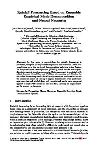
The computations based on adaptive wavelets have been performed using the package fit3 developed in [Casta˜ no (2005)]. 2.5. Numerical experiments In order to assess the quality of the three different EMD schemes, we compare them using a synthetic bivariate example function, see Figure 1, additively composed as the sum of a fast (fstrd1 ) and a slowly oscillating cosine function (fstrd2 ). The function fstrd := fstrd1 + fstrd2 is evaluated on a uniform grid with 200 points in each coordinate direction. We then construct for the three different approaches the empirical mode decomposition according to Algorithm 1 with the modification of Step (3) in the wavelet-nD-case. We expect that the first two intrinsic mode functions are in fact the two components of the test function: the first one should catch the faster frequencies and the second the slower ones. First we see in Figure 2 the result using linear finite elements (FE). Displayed are the first two intrinsic mode functions, imf1 and imf2 and, additionally, the deviation of the second (slowly oscillating) component of fstrd to imf2 . This low oscillatory component fstrd2 has proved to be more difficult to be extracted correctly. We notice that the method based on linear FE fails to correctly represent imf2 as the second component of the test function. We see the results of the corresponding experiment using thin-plate-splines in Figure 3 and adaptive spline-wavelets in Figure 4. We conclude that the quality of the approximation using the FE method is not satisfactory. In contrast, the ThP method and the Wav scheme provide a correct extraction of both imf components, in particular, imf2 . After considering the quality of reconstruction, we next need to compare computational times. Adaptive methods usually require more sophisticated data structures

April 15, 2010

10

19:42

hht-nd

G. Jager, R. Koch, A. Kunoth and R. Pabel

Fig. 1. Test function fstrd (top), composed as the sum from fstrd1 (middle) and fstrd2 (bottom).

because of their inherent hierarchy which might be disadvantageous when comparing speeds. We have measured computational times in seconds for the complete

April 15, 2010

19:42

hht-nd

Fast EMD of Multivariate Data Based on Adaptive Spline-Wavelets

11

EMD algorithms using the three different methods when increasing the number of points in Xf in each coordinate direction. For the FE method, we have for this example used an algorithm based on the techniques developed in [Kobbelt et al. (1998)] for which optimal linear complexity O(N ) for the total number of points N was established. The result is displayed in Figure 5 for a Intel(R) Core(TM) 2 CPU with 2.40 GHz. All programs were implemented in C++. We notice that the linear Finite Elements (FE) and the adaptive wavelet scheme have similar costs with a very slight advantage of the Wav algorithm. Specifically, this plot confirms the optimal linear complexity of the adaptive wavelet scheme. The thin-plate spline approach is much more expensive on account of the globally supported basis functions; note the logarithmic scale in the time direction. Since the linear FE method fails due to unsatisfactory reconstruction and the thin-plate-spline approach is too expensive, as we have seen for this simple synthetic example, we will consider from now on only the adaptive wavelet-nD-EMD. Finally, we investigate the influence of the thresholding parameter ε1 controlling the inner iteration in Step (5) of Algorithm 1. We consider a test image gstrd constructed as the sum of two images with fast and slowly oscillating features gstrd1 and gstrd2 respectively, see Figure 6. We compute the adaptive wavelet-nD-EMD for different values of ε1 . Again we expect that the first two resulting intrinsic mode functions are similar to the two components of the test function. We can get an idea of the quality of the decomposition by looking at the second, slower frequency component. We have found that the quality of the resulting imfs depends strongly on how the thresholding parameter ε1 is chosen. Figure 7 shows in each row the first two intrinsic mode functions for different values of ε1 . The top row displays the result for a very good choice ε1 = 0.02. Here, the number of inner iterations in Algorithm 1 was k = 13 for the first imf and k = 6 for the second imf. A too large parameter like ε1 = 0.2 results in an insufficient reconstruction, as shown in the second row. Here the number of interior iterations was only k = 2 and k = 1 for the first and second imf, respectively. For this value of ε1 , the algorithm exits from the inner loop prematurely and the resulting imf contains too little information from the signal. Choosing the parameter too small, e.g., ε1 = 0.009 displayed in the bottom row, additional oscillations, noise or artefacts are introduced. Moreover, this costs many more inner iterations: k = 200 for the first imf and k = 48 for the second imf. Also, in both cases, the relative errors of the imf to the specific components of the test function increase when deviating too far from the optimal range which is for this example ε ∈ (0.02, 0.03). Further experiments including the choice of the weight parameter α in (7) can be found in [Koch (2008)].

April 15, 2010

12

19:42

hht-nd

G. Jager, R. Koch, A. Kunoth and R. Pabel

Fig. 2. Empirical mode decomposition of test function fstrd using linear Finite Elements (FE): the first two intrinsic mode functions imf1 (top) and imf2 (middle) and the deviation of the second component of the test function fstrd2 to the second intrinsic mode function imf2 (bottom).

April 15, 2010

19:42

hht-nd

Fast EMD of Multivariate Data Based on Adaptive Spline-Wavelets

13

Fig. 3. Empirical mode decomposition of test function fstrd using thin-plate splines (ThP); arrangements of plots as in Figure 2.

April 15, 2010

14

19:42

hht-nd

G. Jager, R. Koch, A. Kunoth and R. Pabel

Fig. 4. Empirical mode decomposition of test function fstrd using adaptive spline wavelets (Wav): arrangement of plots as in Figure 2.

April 15, 2010

19:42

hht-nd

Fast EMD of Multivariate Data Based on Adaptive Spline-Wavelets

15

4

10

WAV FE THP

3

10

time (sec.)

2

10

1

10

0

10

−1

10

0

20

40

60

80

100

120

140

160

180

200

number of unknowns in each direction

Fig. 5. Computation time using linear Finite Elements (FE), Thin-Plate splines (ThP) and adaptive spline wavelets (Wav) when increasing the number of unknowns in each coordinate direction.

20

1.5

40

20

0.8

20

0.8

40

0.6

40

0.6

60

0.4

60

0.4

80

0.2

80

0.2

1 60 0.5

80 100

0

120

−0.5

140

100

0

100

0

120

−0.2

120

−0.2

140

−0.4

140

−0.4

160

−0.6

160

−0.6

180

−0.8

180

−1 160 −1.5

180 200

20

40

60

80

100

120

140

160

180

200

200

20

40

60

80

100

120

140

160

180

200

200

−0.8

20

40

60

80

100

120

140

160

180

Fig. 6. Test function gstrd (left), composed from gstrd1 (middle) and gstrd2 (right).

200

April 15, 2010

16

19:42

hht-nd

G. Jager, R. Koch, A. Kunoth and R. Pabel

1 20 1

40 60

0.5

80 100

20

0.8

40

0.6

60

0.4 0.2

80

0

100

−0.2

0 120

120 −0.4

140

140 −0.6

−0.5 160

160 −0.8

180

180

−1

−1 200

20

40

60

80

100

120

140

160

180

200

200

20

20

40

60

80

100

120

140

160

180

200

2

20 1

40

40

60

0.5

1.5

60 1

80

80 0

100 120

0.5

100 120

0

−0.5 140

140 −0.5

160

−1

180

160 −1

180 −1.5

200

20

40

60

80

100

120

140

160

180

200

200

20

40

60

80

100

120

140

160

180

200

1 20

20 0.8

1 40

40

60

60

0.6 0.4

0.5 80

80

100

100

0.2 0

0 120

120

−0.2

140

−0.4

160

160

−0.6

180

180

−0.8

140 −0.5

−1 200

20

40

60

80

100

120

140

160

180

200

200

−1 20

40

60

80

100

120

140

160

180

200

Fig. 7. Adaptive wavelet-nD-EMD for ε1 = 0.02 (top row), ε1 = 0.2 (middle row) and ε1 = 0.009 (bottom row): the first two intrinsic mode functions imf1 and imf2 .

April 15, 2010

19:42

hht-nd

Fast EMD of Multivariate Data Based on Adaptive Spline-Wavelets

17

3. Generalization of Hilbert Spectral Analysis 3.1. Monogenic signals Once the data is decomposed into an nD-EMD according to (1), one can compute from each component imfj a monogenic signal. This is a multivariate generalization of the complexification of a real-valued one-dimensional function in terms of the Hilbert transform which has a long tradition in signal analysis, see, e.g., [Hahn (1995)]. For univariate functions, this allows one to define instantaneous (locationdependent) frequencies and amplitudes and a corresponding Hilbert spectrum. For functions living on two-dimensional domains like images, a corresponding generalization enables to define local amplitude, orientation and phase functions. This has been developed in [Felsberg and Sommer (2001)] for n = 2 and for the case of general space dimension n in [Felsberg and Sommer (2000)]. The natural generalization leads to Clifford-algebra-valued functions and, for n = 2, to quaternions. We follow this construction which we briefly summarize here. Starting from the decomposition (1), we therefore compute from each nD component imfj a monogenic signal imfjM (x) := imfj (x) + imfjH (x)e1

where imfjH := imfj ∗hn .

(12)

Here e1 ∈ Rn is the first unit vector. The function hn is the convolution kernel of the Riesz transform, a multivariate generalization of the Hilbert transform, and is given by hn (x) := cn

x e1 , kxkn+1

(13)

where cn is an explicitly known constant depending on the spatial dimension n. Practically, a monogenic signal can be computed by applying Hilbert and Radon transforms. For q a monogenic signal fM , one can define a local amplitude function

a(fM )(x) := fM (x) fM (x), a phase function φ(fM )(x) := arg(fM (x)) ∈ [0, 2π) and orientation functions θ1 , . . . , θn−1 ∈ [0, π), see [Felsberg and Sommer (2000)]. Based on the representation (1) and the manipulation (12) for each imfj , we define the cumulative monogenic signal of f : Ω → R as fkum (x) :=

J X

imfjM (x) =

j=1

J X (imfj (x) + imfjH (x) e1 ).

(14)

j=1

For this cumulative function we can assemble an orientation vector based on the local orientations θ := (θ1 , . . . , θn−1 )T of each nD intrinsic mode function as 

 θ(imf1M )(x)   .. J(n−1) θ(fkum )(x) :=  , ∈R . θ(imfJM )(x)

(15)

April 15, 2010

18

19:42

hht-nd

G. Jager, R. Koch, A. Kunoth and R. Pabel

and similarly a phase and amplitude vector of the cumulative function,     a(imf1M )(x) φ(imf1M )(x)     .. .. J J a(fkum )(x) :=  φ(fkum )(x) :=  ∈R . ∈R ; . . φ(imfJM )(x)

a(imfJM )(x) (16)

3.2. Numerical experiment Specifically the local amplitude can be used for two-dimensional images to detect local edges since it only reacts at edges and vanishes otherwise. In order to show agreement with existing results and interpretations in the literature [Felsberg and Sommer (2001)], we will show this in the following numerical experiment for a bivariate function. We display in Figure 8 a composed image on the left and on the right the amplitude functions of the corresponding monogenic signal. One can see from the latter strong oscillating features on the finest scale. The amplitude function reacts at the edges and vanishes otherwise. We decompose the image on the left using the adaptive wavelet-2d-EMD and find eleven 2d-imfs and a residual. The first imf1 can be seen in Figure 9 on the left together with the amplitude function of the corresponding monogenic signal on the right. We clearly see that imf1 contains the components on the finest scale.

Fig. 8. Composed original image (left) and amplitude function of the corresponding monogenic signal (right).

The second 2D-imf describes the function part on the next coarser intrinsic scale. It is displayed in Figure 10 on the top left together with the local amplitude function (top right), the local orientation function (bottom left) and the local phase function (bottom right) of the corresponding monogenic signal. One can see that the local amplitude function is only visible after the decomposition into the inherent pattern on a coarser scale, the circular structure. The local orientation function

April 15, 2010

19:42

hht-nd

Fast EMD of Multivariate Data Based on Adaptive Spline-Wavelets

19

Fig. 9. First 2D-imf1 of the EMD (left) and amplitude function of the corresponding monogenic signal (right).

displays edges and one-dimensional subspaces orthogonal to locally constant directions. Finally, the local phase shows symmetries of the inherent one-dimensional local functions in the direction of the one-dimensional subspaces described by the local orientations. These results and interpretations are in perfect accordance to previously made observations [Felsberg and Sommer (2001); Nunes and Del´echelle (2009)]. This shows that the imfs from our adaptive wavelet nD-EMD are perfectly suited for image analysis using monogenic signals as previously used EMD methods.

4. Conclusions We have presented a general setup for an n–dimensional empirical mode decomposition. In order to obtain a method with optimal complexity, we have combined a method based on local means with an adaptive wavelet data fitting procedure. We compared our method with a scheme based on finite elements and a method based on thin-plate-splines and found it superior both with respect to the quality of the reconstruction and the speed of computations. Specifically, our method has been shown to be of optimal linear complexity. We also studied the decomposition quality when changing the relevant stopping parameter in the EMD process. Computing afterwards via monogenic signals of each nD-imf a cumulative function, we can extract local amplitude, orientation and phase functions and find our results in perfect agreement with previously published results from image analysis.

Acknowledgment We gratefully acknowledge financial support by the SFB/TR 32 “Pattern in SoilVegetation-Atmosphere Systems: Monitoring, Modelling, and Data Assimilation” www.tr32.de, funded by the Deutsche Forschungsgemeinschaft (DFG).

April 15, 2010

20

19:42

hht-nd

G. Jager, R. Koch, A. Kunoth and R. Pabel

Fig. 10. Second 2D-imf2 of the EMD (top left); amplitude function (top right), orientation function (bottom left) and phase function (bottom right) of the corresponding monogenic signal.

References Buhmann, M.D. (2003). Radial Basis Functions: Theory and Implementations. Cambridge University Press. Bhuiyan, S.M.A. and Attoh-Okine, N.O. and Barner, K.E. and Ayenu-Prah, A.Y. and Adhami, R.R. (2009). Bidimensional empirical mode decomposition using various interpolation techniques. Adv. in Adap. Data Anal., 1:309–338. Casta˜ no, D. (2005). Adaptive Scattered Data Fitting with Tensor Product Spline– Wavelets. Doctoral Dissertation, Universit¨ at Bonn. Casta˜ no, D. and Kunoth, A. (2003). Adaptive fitting of scattered data by spline–wavelets. Curves and Surfaces, eds. L.L. Schumaker et. al., Vanderbilt University Press, pp. 65– 78. Casta˜ no, D. and Kunoth, A. (2006). Robust regression of scattered data with adaptive spline-wavelets. IEEE Trans. Image Proc., 15 (6):1621–1632. Chan, W.L. and Choi, H. and Baraniuk, R.G. (2008) Coherent multiscale image processing using dual-tree quaternion wavelets. IEEE Trans. Image Proc., 17 (7):1069–1082. Chen, Q. and Huang, N. E. and Riemenschneider, S. and Xu, Y. (2006) A B-spline approach for empirical mode decomposition. Adv. Comput. Math., 24:171–195. Damerval, Ch. and Meignen, S. and Perrier, V. (2005). A fast algorithm for bidimensional EMD IEEE Signal Process. Lett., 12(10):701–704. Del´echelle, E. and Lemoine, J. and Niang, O. (2005). Empirical mode decomposition: An analytical approach for sifting process. IEEE Signal Process. Lett., 12(11):764–767.

April 15, 2010

19:42

hht-nd

Fast EMD of Multivariate Data Based on Adaptive Spline-Wavelets

21

Felsberg, M. (2002) Low-Level Image Processing with the Structure Multivector. Doctoral Dissertation, Universit¨ at Kiel. Felsberg, M. and Sommer, G. (2000). The multidimensional isotropic generalization of quadrature filters in geometric algebra. Lecture Notes in Computer Science, 1888:175– 185. Felsberg, M. and Sommer, G. (2001). The monogenic signal. IEEE Transactions on Signal Proc., 49:3136–3144. Flandrin, P. and Gon¸calv`es, P. (2004). Empirical mode decompositions as data-driven wavelet-like expansions. Int. J. Wavelets Multiresolut. Inform. Process., 2:477–496. Hahn, S. (1995) Hilbert Transforms in Signal Processing. Artech House. Held, S. and Storath, M. and Massopust, P. and Forster, B. (2010). Steerable wavelet frames based on the Riesz transform. To appear in IEEE Transactions on Image Processing. Huang, Y.X. and Schmitt, F.G. and Lu, Z.M. and Liu, Y.L. (2009). Analysis of daily river flow fluctuations using empirical mode decomposition and arbitrary order Hilbert spectral analyis. Journal of Hydrology, 373:103–111. Huang, N.E. and Shen, Z. and Long, S.R. and Wu, M.C. and Shih, H.H. and Zhang, Q. and Yen, N.-C. and Tung, C.C. and Liu, H.H (1998). The empirical mode decomposition and the Hilbert spectrum for nonlinear and non-stationary time series analysis. Proc. R. Soc. Lond. A, 454:903–995. Huang, N.E. and Shen, S.S.P. (2005) Hilbert-Huang Transform and its Applications. World Scientific Publishing. Koch, R. (2008). Analyse multivariater Daten: Konstruktion monogener Clifford–Algebra– wertiger Funktionen mittels Empirical Mode Decomposition basierend auf adaptiven kubischen Spline-Wavelets und der Riesz-Transformation (in German). Diplomarbeit, Institut f¨ ur Numerische Simulation, Universit¨ at Bonn. Kobbelt, L. and Campagna, S. and Vorsatz, J. and Seidel, H.-P. (1998) Interactive multiresolution modeling on arbitrary meshes. Proc. Siggraph pp. 105-144. J. Rudi and R. Pabel and G. Jager and R. Koch and A. Kunoth and H. Bogena (2010). Multiscale analysis of hydrologic time series data using the Hilbert-Huang-Transform (HHT). To appear in Vadose Zone Journal. Linderhed, A. (2004) Image compression based on empirical mode decomposition. Proceedings of SSAB 04 Symposium on Image Analysis pp. 110–113. Linderhed, A. (2009) Image empirical mode decomposition: A new tool for image processing. Adv. in Adap. Data Anal., 1:265-294. Liu, Z. and Peng, S. (2002). Directional EMD and its application to texture segmentation. Science in China (Series F), 45(12):1–11. Nunes, J.C. and Niang, O. and Bouaoune, Y. and Del´echelle, E. and Bunel, Ph. (2003). Bidimensional empirical mode decomposition modified for texture analysis. Lecture Notes in Computer Science, 2749:171–177. Nunes, J.C. and and Del´echelle, E. (2009). Empirical mode decomposition: Applications on signal and image processing. Adv. in Adap. Data Anal., 1:125–175. Rilling, G. and Flandrin, P. and Gon¸calv`es, P. and Lilly, J.M. (2007). Bivariate empirical mode decompositions. IEEE Sig. Proc. Lett. , 14(12):936–939. Sharpley, R. C. and Vatchev, V. (2006) Analysis of the intrinsic mode functions. Constr. Approx., 24 (1):14–47. Stollnitz, E.J. and DeRose, T.D. and Salesin, D. (1996). Wavelets for Computer Graphics: Theory and Applications. Morgan Kaufman. Titchmarsh, E.C. (1950) Introduction into the Theory of Fourier Integral. Oxford University Press.

April 15, 2010

22

19:42

hht-nd

G. Jager, R. Koch, A. Kunoth and R. Pabel

Wietzke, L. and Sommer, G. and Schmaltz, C. (2009). The conformal monogenic signal of image sequences. Statistical and Geometrical Approaches to Visual Motion Analysis. eds. D. Cremers et al., LNCS 5604, Springer, pp. 305–322. Wu, Z. and Huang, N.E. and Chen, X. (2009). The multi-dimensional ensemble empirical mode decomposition method. Adv. in Adap. Data Anal., 1:339–371. Xu, Y. and Liu, B. and Liu, J. and Riemenschneider, S. (2006). Two-dimensional empirical mode decomposition by finite elements. Proc. R. Soc. Lond. A, 462:3081–3096. Yuan, Y. and Jing, M. and Song, P. and Zhang, J. (2009). Empiric and dynamic detection of the sea bottom topography from synthetic aperture radar image. Adv. in Adap. Data Anal., 1:243–263.