Energies 2013, 6, 1887-1901; doi:10.3390/en6041887 OPEN ACCESS
energies ISSN 1996-1073 www.mdpi.com/journal/energies Article
Support Vector Regression Model Based on Empirical Mode Decomposition and Auto Regression for Electric Load Forecasting Guo-Feng Fan 1, Shan Qing 1,*, Hua Wang 1, Wei-Chiang Hong 2 and Hong-Juan Li 1 1
2
Engineering Research Center of Metallurgical Energy Conservation and Emission Reduction, Ministry of Education, Kunming University of Science and Technology, Kunming 650093, China; E-Mails:
[email protected] (G.-F.F.);
[email protected] (H.W.);
[email protected] (H.-J.L.) Department of Information Management, Oriental Institute of Technology/58 Sec. 2, Sichuan Rd., Panchiao, Taipei 220, Taiwan; E-Mail:
[email protected]
* Author to whom correspondence should be addressed; E-Mail:
[email protected]; Tel.: +86-1388-855-2395; Fax: +86-0871-6515-3405. Received: 28 November 2012; in revised form: 2 February 2013 / Accepted: 25 March 2013 / Published: 2 April 2013
Abstract: Electric load forecasting is an important issue for a power utility, associated with the management of daily operations such as energy transfer scheduling, unit commitment, and load dispatch. Inspired by strong non-linear learning capability of support vector regression (SVR), this paper presents a SVR model hybridized with the empirical mode decomposition (EMD) method and auto regression (AR) for electric load forecasting. The electric load data of the New South Wales (Australia) market are employed for comparing the forecasting performances of different forecasting models. The results confirm the validity of the idea that the proposed model can simultaneously provide forecasting with good accuracy and interpretability. Keywords: electric load prediction; support vector regression; empirical mode decomposition auto regression
1. Introduction Electric energy is an unstored resource, thus, electric load forecasting plays a vital role in the management of the daily operations of a power utility, such as energy transfer scheduling, unit
Energies 2013, 6
1888
commitment, and load dispatch. With the emergence of load management strategies, it is highly desirable to develop accurate, fast, simple, robust and interpretable load forecasting models for these electric utilities to achieve the purposes of higher reliability and better management [1]. In the past decades, researchers have proposed lots of methodologies to improve load forecasting accuracy. For example, Bianco et al. [2] proposed linear regression models for electricity consumption forecasting; Zhou et al. [3] applied a grey prediction model for energy consumption; Afshar and Bigdeli [4] proposed an improved singular spectral analysis method for short-term load forecasting (STLF) for the Iranian electricity market; and Kumar and Jain [5] applied three time series models—Grey-Markov model, Grey-Model with rolling mechanism, and singular spectrum analysis—to forecast the consumption of conventional energy in India. By employing artificial neural networks, references [6–9] proposed several useful short-term load forecasting models. By hybridizing the popular method and evolutionary algorithm, the authors of [10–13] demonstrated further performance improvements which could be made for energy forecasting. Though these methods can yield a significant proven forecasting accuracy improvement in some cases, they have usually focused on the improvement of the accuracy without paying special attention to the interpretability. Recently, expert systems, mainly developed by means of linguistic fuzzy rule-based systems, allow us to deal with the system modeling with good interpretability [14]. However, these models have strong dependency on an expert and often cannot generate good accuracy. Therefore, combination models, based on the popular methods, expert systems and other techniques, are proposed to satisfy both high accurate level and interpretability. Based on the advantages in statistical learning capacity to handle high dimensional data, the SVR (support vector regression) model, especially suitable for small sample size learning, has become a popular algorithm for many forecasting problems [15–17]. As a disadvantage of an SVR method, it is easily trapped into a local optimum during the nonlinear optimization process of the three parameters, in the meanwhile, its robustness and sparsity are also lacking satisfactory levels. On the other hand, empirical mode decomposition (EMD) and auto regression (AR), a fast, easy and reliable unsupervised clustering algorithm, has been successfully applied to many fields, such as communication, society, economy, engineering, and has achieved good effects [18–20]. Particularly, the EMD method can effectively extract the components of the basic mode from nonlinear or non-stationary time series [21], i.e., the original complex time series can be transferred into a series of single and apparent components. It can effectively reduce the interactions among lots of singular values and improve the forecasting performance of a single kernel function. Thus, it is useful to employ suitable kernel functions for forecasting the medium-and-long-term tendencies of the time series. In this paper, we present a new hybrid model with clear human-understandable knowledge on training data to achieve a satisfactory level of forecasting accuracy. The principal idea is hybridizing EMD with SVR and AR, namely creating the EMDSVRAR model, to receive better solutions. The proposed EMDSVRAR model has the capability of smoothing and reducing the noise (inherited from EMD), the capability of filtering dataset and improving forecasting performance (inherited from SVR), and the in capability of effectively forecasting the future tendencies of data (inherited from AR). The forecasting outputs of an unseen example by using the hybrid method are described in the following section. To show the applicability and superiority of the proposed algorithm, half-hourly electric load data (48 data points per day) from New South Wales (Australia) with two different sample sizes are
Energies 2013, 6
1889
employed to compare the forecasting performances among the proposed model and other four alternative models, namely the PSO-BP model (BP neural network trained by a particle swarm optimization algorithm), SVR model, PSO-SVR model (optimal combination of SVR parameters determined by a PSO algorithm), and the AFCM model (an adaptive fuzzy combination model based on a self-organizing map and support vector regression). This study also suggests that researchers and practitioners should carefully consider the nature and intention in using these electric load data while neural networks, statistical methods, and other hybrid models are being determined to be the critical management tools in electricity markets. The experimental results indicate that this proposed EMDSVRAR model has the following advantages: (1) simultaneously satisfies the need for high levels of accuracy and interpretability; (2) the proposed model can tolerate more redundant information than the original SVR model, thus, it has better generalization ability. The rest of this paper is organized as follows: in Section 2, the EMDSVRAR forecasting model is introduced and the main steps of the model are given. In Section 3, the data description and the research design are outlined. The numerical results and comparisons are presented and discussed in Section 4. A brief conclusion of this paper and the future research are provided in Section 5. 2. Support Vector Regression with Empirical Mode Decomposition 2.1. Empirical Mode Decomposition (EMD) The EMD method is based on the simple assumption that any signal consists of different simple intrinsic modes of oscillations. Each linear or non-linear mode will have the same number of extreme and zero-crossings. There is only one extreme between successive zero-crossings. Each mode should be independent of the others. In this way, each signal could be decomposed into a number of intrinsic mode functions (IMFs), each of which should satisfy the following two definitions [22]: a In the whole data set, the number of extreme and the number of zero-crossings should either equal or differ to each other at most by one. b At any point, the mean value of the envelope defined by local maxima and the envelope defined by the local minima is zero. An IMF represents a simple oscillatory mode compared with the simple harmonic function. With the definition, any signal x(t ) can be decomposed as following steps: 1 Identify all local extremes, and then connect all the local maxima by a cubic spline line as the upper envelope. 2 Repeat the procedure for the local minima to produce the lower envelope. The upper and lower envelopes should cover all the data among them. 3 The mean of upper and low envelope value is designated as m1 , and the difference between the signal x(t ) and m1 is the first component, h1 , as shown in Equation (1): h1 = x(t ) − m1 (1) Generally speaking, h1 will not necessarily meet the requirements of the IMF, because h1 is not a standard IMF. It needs to be determined for k times until the mean envelope tends to zero. Then, the
Energies 2013, 6
1890
first intrinsic mode function c1 is introduced, which stands for the most high-frequency component of the original data sequence. At this point, the data could be represented as Equation (2): h1k = h1( k −1) − m1k
(2)
where h1k is the datum after k times siftings. h1( k −1) stands for the data after k − 1 times sifting. Standard deviation ( SD ) is used to determine whether the results of each filter component meet the IMF or not. SD is defined as Equation (3): T
SD = k =1
h1( k −1) (t ) − h1k (t )
2
h1(2 k −1) (t )
(3)
where T is the length of the data. The value of standard deviation SD is limited in the range of 0.2 to 0.3, which means when 0.2 < SD < 0.3 , the decomposition process can be finished. The consideration for this standard is that it should not only ensure hk (t ) to meet the IMF requirements, but also control the decomposition times. Therefore, in this way, the IMF components could retain amplitude modulation information in the original signal. 4 When h1k has met the basic requirements of SD , based on the condition of c1 = h1k , the signal x(t ) of the first IMF component c1 can be obtained directly, and a new series r1 could be achieved after deleting the high frequency components. This relationship could be expressed as Equation (4): r1 = x(t ) − c1
(4)
The new sequence is treated as the original data and repeats the steps (1) to (3) processes. The second intrinsic mode function c2 could be obtained. 5 Repeat previous steps (1) to (4) until the rn can not be decomposed into the IMF. The sequence rn is called the remainder of the original data x(t ) . rn is a monotonic sequence, it can indicate the overall trend of the raw data x(t ) or mean, and it is usually referred as the so-called trend items. It is of clear physical significance. The process is expressed as Equations (5) and (6): r1 = x(t ) − c1 , r2 = r1 − c2 , , rn = rn −1 − cn
(5)
n
x(t ) = ci + rn i =1
(6)
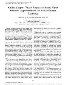
The original data can be expressed as the IMF component and remainder. 2.2. Support Vector Regression The notions of SVMs for the case of regression are introduced briefly. Given a data set of N elements {( X i , yi ), i = 1, 2, , N } , where X i is the i-th element in n-dimensional space, i.e., X i = [ x1i , , xni ] ∈ ℜn , and yi ∈ ℜ is the actual value corresponding to X i . A non-linear mapping (·): ℜn → ℜnh is defined to map the training (input) data X i into the so-called high dimensional feature space (which may have infinite dimensions), ℜnh (Figure 1a,b). Then, in the high dimensional feature
Energies 2013, 6
1891
space, there theoretically exists a linear function, f , to formulate the non-linear relationship between input data and output data. Such a linear function, namely SVR function, is shown as Equation (7):
f ( X ) = W Tϕ ( X ) + b
(7)
where f ( X ) denotes the forecasting values; the coefficients W ( W ∈ ℜnh ) and b ( b ∈ ℜ ) are adjustable. As mentioned above, the SVM method aims at minimizing the empirical risk, shown as Equation (8): 1 Remp ( f ) = N
N
Θε ( y , W i
T
ϕ ( X i ) + b)
(8)
i =1
where Θε ( y, f ( x)) is the ε-insensitive loss function (indicated as a thick line in Figure 1c) and defined as Equation (9): f ( X ) − Y − ε , if f ( X ) − Y ≥ ε Θε (Y , f ( X )) = otherwise 0,
(9)
Figure 1. Transformation process illustration of a SVR model. (a) Input space; (b) Feature space; (c) ε-insensitive loss function.
(a) ϕ(X ) +ε
ξ
* i
−ε
ξi Input space
ξ i* •
ε−
In addition, Θε (Y , f ( X )) is employed to find out an optimum hyperplane on the high dimensional feature space (Figure 1b) to maximize the distance separating the training data into two subsets. Thus, the SVR focuses on finding the optimum hyper plane and minimizing the training error between the
Energies 2013, 6
1892
training data and the ε -insensitive loss function. Then, the SVR minimizes the overall errors, shown as Equation (10): N 1 Min∗ Rε (W , ξ ∗ , ξ ) = W TW + C (ξi∗ + ξi ) W ,b ,ξ ,ξ 2 i =1
(10)
with the constraints: Yi − W T ϕ ( X i ) − b ≤ ε + ξi∗ , −Yi + W T ϕ ( X i ) + b ≤ ε + ξi , ξi* ≥ 0, ξi ≥ 0,
i = 1, 2,..., N i = 1, 2,..., N i = 1, 2,..., N i = 1, 2,..., N
(11)
The first term of Equation (10), employing the concept of maximizing the distance of two separated training data, is used to regularize weight sizes to penalize large weights, and to maintain regression function flatness. The second term penalizes training errors of f ( x) and y by using the ε -insensitive loss function. C is the parameter to trade off these two terms. Training errors above ε are denoted as ξi∗ , whereas training errors below − ε are denoted as ξi (Figure 1b). After the quadratic optimization problem with inequality constraints is solved, the parameter vector w in Equation (7) is obtained as Equation (12): N
W = ( β i∗ − βi )ϕ ( X i ) i =1
(12)
where ξi∗ , ξi are obtained by solving a quadratic program and are the Lagrangian multipliers. Finally, the SVR regression function is obtained as Equation (13) in the dual space: N
f ( X ) = ( β i∗ − β i ) K ( X i , X ) + b i =1
(13)
where K ( X i , X ) is called the kernel function, and the value of the kernel equals the inner product of two vectors, X i and X j , in the feature space ϕ ( X i ) and ϕ ( X j ) , respectively; that is, K ( X i , X j ) = ϕ ( X i )ϕ ( X j ) . Any function that meets Mercer’s condition [23] can be used as the kernel function. There are several types of kernel function. The most used kernel functions are the Gaussian radial 2 basis functions (RBF) with a width of σ : K ( X i , X j ) = exp(−0.5 X i − X j / σ 2 ) and the polynomial kernel with an order of d and constants a1 and a2 : K ( X i , X j ) = (a1 X i X j + a2 ) d . However, the Gaussian RBF kernel is not only easy to implement, but also capable of non-linearly mapping the training data into an infinite dimensional space, thus, it is suitable to deal with non-linear relationship problems. Therefore, the Gaussian RBF kernel function is specified in this study. The forecasting process of a SVR model is illustrated in Figure 2.
Energies 2013, 6
1893 Figure 2. The forecasting process of a SVR model.
K ( X , X1 )
K(X , X2 )
β1 − β1*
K(X , X3 )
K(X , X5 )
K(X , X4 )
* * β 2 − β 2* β3 − β3 β 4 − β 4 β5 − β
K(X , XN )
* 5
βi − β i*
β N − β N*
N
f (X, β , β * ) = ( βi , βi* )K (X,Xi ) + b i =1
2.3. AR Model Equation (14) expresses a p -step autoregressive model, referring as AR( p) model [24]. Stationary time series { X t } that meet the model AR( p) is called the AR( p) sequence. That a = (a1 , a2 , , a p )T is named as the regression coefficients of the AR( p) model: p
X t = a j X t− j + εt , t ∈ Z
(14)
j =1
3. Numerical Examples
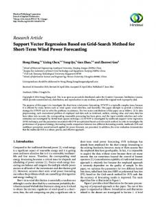
In the first experiment, the proposed model is trained by electric load from New South Wales (Australia) from 2 May 2007 to 7 May 2007, and testing electric load is from 8 May 2007. The employed electric load data is on a half-hourly basis (i.e., 48 data points per day). The data size contains only 7 days, to differ from the other example with more sample data, this example is so-called the small sample size data, and illustrated in Figure 3a.
11000
11000
10000
10000
9000
9000
8000
8000
7000
7000
6000 5000
Original data EMD data-I
4000 3000 2000
Electric load (MW)
Electric load (MW)
Figure 3. (a) Half-hourly electric load in New South Wales from 2 May 2007 to 8 May 2007; (b) Half-hourly electric load in New South Wales from 2 May 2007 to 24 May 2007.
6000 5000
Original data EMD data-I
4000 3000 2000 1000
1000
0
0
-1000
-1000
-2000 -3000
-2000 -50
0
50
100
150
200
Time (half hour)
(a)
250
300
350
0
200
400
600
Time (half hour)
(b)
800
1000
1200
Energies 2013, 6
1894
Too large training sets should avoid overtraining during the learning process of the SVR model. Therefore, the second experiment with 23 days (1104 data points from 2 May 2007 to 24 May 2007) is modeled by using part of all the training samples as training set. This example is so-called the large sample size data, and illustrated in Figure 3b. 3.1. Results after EMD After being decomposed by EMD, the data can be divided into eight groups, which are shown in Figure 4a–h and the last group (Figure 4h) is a trend term (remainders). The so-called high frequency item is obtained by adding the preceding seven groups. From Figures 3a,b, the trend of the high frequency item is the same as original data, and its the structure is more regular, i.e., it is more stable. Then, the high frequency item (data-I) and the remainders (data-II) have good effect of regression by the SVR and AR, respectively, and will be described as follow. Figure 4. For ease of prevention, the graphs (a–h) show our section of plots at different IMFs for the small sample size. 2500 2000 1000
a
2000
1000
500 0
Electric load (MW)
1000
c
1500
500
Electric load (MW)
Electric load (MW)
1500
b
0
-500
-500
500 0 -500 -1000 -1500
-1000
-1000
-2000 0
50
100
150
200
250
300
0
50
100
Time (half hour)
150
200
250
300
0
50
100
Time (half hour)
150
200
250
300
Time (half hour) 200
1500
1000
d
0 -500 -1000
150
e
500
0
-500
f
100
Electric load (MW)
500
Electric load (MW)
Electric load (MW)
1000
50 0 -50 -100
-1000 -1500
-150
-2000
-1500 0
50
100
150
200
250
300
-200 0
50
100
Time (half hour)
150
200
250
300
0
50
100
Time (half hour)
150
200
250
300
250
300
Time (half hour)
8700
11000
80 8600
g
20 0 -20 -40
8400 8300 8200 8100
-60
10000
h
8500
Electric load (MW)
Electric load (MW)
40
Electric load (MW)
60
8000
9000
8000
7000
6000
-80 7900 0
50
100
150
200
Time (half hour)
250
300
0
50
100
150
200
Time (half hour)
250
300
0
50
100
150
200
Time (half hour)
Energies 2013, 6
1895
3.2. Forecasting Using SVR for Data I (The High Frequency Item) Firstly, for both small sample and large sample data, the high-frequency item is simultaneously employed for SVR modeling, and the better performances of the training and testing (forecasting) sets are shown in Figure 5a,b, respectively. The correlation coefficients of training effects are 0.9912 and 0.9901, respectively, of the forecast effects are 0.9875 and 0.9887, accordingly. This implies that the decomposition is helpful to improve the forecasting accuracy. The parameters of a SVR model for data I are shown in Table 1. Figure 5. Comparison of the data-I and the forecasted electric load of train and test by the SVR model for the small sample and large sample data: (a) One-day ahead prediction of 8 May 2007 are performed by the model; (b) One-week ahead prediction from 18 May 2007 to 24 May 2007 are performed by the model.
(a)
(b)
Table 1. The SVR’s parameters for data-I and data-II. Sample size The high frequency item (data-I) The remainders (data-II)
m 20 20
σ 0.1 0.35
C 100 181
ε 0.0061 0.0034
Testing MAPE 9.85 5.1
3.3. Forecasting Using AR for Data II (The Remainders) Then, according to the geometric decay of the correlation coefficient and partial correlation coefficients fourth-order truncation for data II (the remainders), it can be regarded as AR (4) model. The parameters of a SVR model for data II are shown in Table 1. As shown in Figure 6a,b, the remainders, for both small sample and large sample data, almost are in a straight line. The good forecasting results are shown in Table 2, and the errors have reached the level of 10−7 for the small or large amount of data. It has demonstrated the superiority of the AR model.
Energies 2013, 6
1896
Figure 6. Comparison of the data-II and the forecasted electric load by the AR model for the two experiments: (a) One-day ahead prediction of 8 May 2007 performed by the model; (b) One-week ahead prediction from 18 May 2007 to 24 May 2007 performed by the model. 8640
Actual Values Predicted Values
8620
9400
Electric load-Trend (MW)
8600
Electric load-Trend(MW)
Actual Values Predicted Values
9500
8580 8560 8540 8520 8500 8480 8460
9300
9200
9100
9000
8900
8440 0
10
20
30
40
50
-50
0
50
100
150
200
250
300
350
Time (half hour)
Time(half hour)
(a)
(b)
Table 2. Summary of results of the AR forecasting model for data-II. Remainders
MAE
Eqution
The small sample size
6.5567 ×10⁻⁷
xn = 8417.298 + 1.013245 xn −1 + 0.490278 xn − 2 −0.011731xn −3 − 0.491839 xn − 4
The large sample size
1.8454 ×10⁻⁷
xn = 8546.869 + 1.000046 xn −1 + 0.499957 xn − 2 −5.18 ×10⁻⁵ xn −3 − 0.499951xn − 4
4. Result and Analysis
This section focuses on the efficiency of the proposed model with respect to computational accuracy and interpretability. To consider the small sample size modeling ability of the SVR model and conduct fair comparisons, we perform a real case experiment with relatively small sample size in the first experiment. The next experiment with 1104 datapoints is focused on illustrating the relationship between sample size and accuracy. 4.1. Parameter Settings of the Employed Forecasting Models As mentioned by Taylor [25], and to be based on the same comparison condition with Wang et al. [26], some parameter settings of the employed forecasting models are set as followings. For the PSO-BP model, we use 90 percent of all training samples as the training set, and the rest as the evaluation set. The parameters used in the PSO-BP are as follows: (i) The first set related to BP neural network: input layer dimension indim = 2, hidden layer dimension hiddennum = 3, output layer dimension outdim = 1; (ii) The second set related to PSO: maximum iteration number itmax = 300, number of particles N = 40, length of particle D = 3, weight c1 = c2 = 2. Because the PSO-SVR model embeds the construction and prediction algorithm of SVR in the fitness value iteration step of PSO, it will take a long time to train the PSO-SVR using the full training dataset.
Energies 2013, 6
1897
For the above reason, we draw a small part of all training samples as training set, and the rest as evaluation set. The parameters used in the PSO are as follows: For small sample size: maximum iteration number itmax = 50, number of particles N = 20, length of particle D = 3, weight c1 = c2 = 2. For large sample size: maximum iteration number itmax = 20, number of particles N = 5, length of particle D = 3, weight c1 = c2 = 2. 4.2. Forecasting Evaluation Methods For the purpose of evaluating the forecasting capability, we examine the forecasting accuracy by calculating three different statistical metrics, the root mean square error (RMSE), the mean absolute error (MAE) and the mean absolute percentage error (MAPE). The definitions of RMSE, MAE and MAPE are expressed as Equations (15–17): n
(P − A ) i
RMSE =
2
i
i =1
(15)
n n
| P − A | i
MAE =
(16)
n n
MAPE =
i
i =1
| i =1
Pi − Ai | Ai *100 n
(17)
Where Pi and Ai are the i-th predicted and actual values respectively, and n is the total number of predictions. 4.3. Empirical Results and Analysis For the first experiment, the forecasting results (the electric load on 8 May 2007) of the original SVR model, the PSO-SVR model and the proposed EMDSVRAR model are shown in Figure 7a. Notice that the forecasting curve of the proposed EMDSVRAR model fits better than other alternative models. The second experiment shows the one-week-ahead forecasting for the large sample size data. The peak load values of testing set are bigger than that of training set shown in Figure 3b. The detailed forecasted results of this experiment are shown in Figure 7b. It indicates that the results obtained from the EMDSVRAR model fits the peak load values exceptionally well. In other words, the EMDSVRAR model has better generalization ability than the three comparison models. The forecasting results from these models are summarized in Table 3. The proposed EMDSVRAR model is compared with four alternative models. It is found that our hybrid model outperforms all other alternatives in terms of all the evaluation criteria. One of the general observations is that the proposed model tends to fit closer to the actual value with a smaller forecasting error.
Energies 2013, 6
1898
Figure 7. Comparison of the original data and the forecasted electric load by the EMDSVRAR Model, the SVR model and the PSO-SVR model for (a) the small sample size (One-day ahead prediction of 8 May 8, 2007 are performed by the models); (b) the large sample size (One-week ahead prediction from May 18, 2007 May 24, 2007 are performed by the models). 12000
11000
Raw data Forecasted load by EMDSVRAR Forecasted load by SVR Forecasted load by PSOSVR
11000 10000
Electric load (MW)
Electric load (MW)
10000 9000
8000
Raw data Forecasted load by EMDSVRAR Forecasted load by SVR Forecasted load by PSOSVR
7000
6000 0
10
20
30
40
50
9000
8000
7000
6000 -50
0
50
100
150
200
Time (half hour)
Time(half hour)
(a)
(b)
250
300
350
The proposed model shows the higher forecasting accuracy in terms of three different statistical metrics. In view of the model effectiveness and efficiency on the whole, we can conclude that the proposed model is quite competitive against four comparison models, the PSO-BP, SVR, PSO-SVR, and AFCM models. In other words, the hybrid model leads to better accuracy and statistical interpretation. Table 3. Summary of results of the forecasting models. Algorithm Original SVR PSO-SVR PSO-BP AFCM [24] EMDSVRAR Original SVR PSO-SVR PSO-BP AFCM [26] EMDSVRAR
MAPE RMSE MAE For the first experiment (small sample size) 11.6955 145.865 10.9181 11.4189 145.685 10.6739 10.9094 142.261 10.1429 9.9524 125.323 9.2588 9.8595 117.159 9.0967 For the second experiment (large sample size) 12.8765 181.617 12.0528 13.503 271.429 13.0739 12.2384 175.235 11.3555 11.1019 158.754 10.4385 5.100 134.201 9.8215
Running Time(s) 180.4 165.2 159.9 75.3 80.7 116.8 192.7 163.1 160.4 162.0
Several observations can also be noticed from the results. Firstly, from the comparisons among these models, we point out that the proposed model outperforms other alternative models. Secondly, the EMDSVRAR model has better generalization ability for different input patterns as shown in the second experiment. Thirdly, from the comparison between the different sample sizes of these two experiments, we conclude that the hybrid model can tolerate more redundant information and construct the model for
Energies 2013, 6
1899
the larger sample size data set. Finally, since the proposed model generates good results with good accuracy and interpretability, it is robust and effective as shown in Table 3. Overall, the proposed model provides a very powerful tool to implement easily for forecasting electric load. Furthermore, to verify the significance of the accuracy improvement of the EMDSVRAR model, the forecasting accuracy comparison among original SVR, PSO-SVR, PSO-BP, AFCM, and EMDSVRAR models is conducted by a statistical test, namely a Wilcoxon signed-rank test, at the 0.025 and 0.05 significance levels in one-tail-tests. The test results are shown in Table 4. Clearly, the proposed EMDSVRAR model has statistical significance (under a significant level 0.05) among the other alternative models, particularly comparing with original SVR, PSO-SVR, PSO-BP, and AFCM models. Table 4. Wilcoxon signed-rank test. Compared models EMD-SVR-AR vs. original SVR EMD-SVR-AR vs. PSO-SVR EMD-SVR-AR vs. PSO-BP EMD-SVR-AR vs. AFCM a
Wilcoxon signed-rank test α = 0.025; W = 4 α = 0.05;W = 6 8 3a 6 2a 6 2a 6 2a
denotes that the EMDSVRAR model significantly outperforms other alternative models.
5. Conclusions
The proposed model achieves superiority and outperforms the original SVR model while forecasting based on the unbalanced data. In addition, the goal of the training model is not to learn an exact representation of the training set itself, but rather to set up a statistical model that generalizes better forecasting values for the new inputs. In practical applications of a SVR model, if the SVR model is overtrained to some sub-classes with overwhelming size, it memorizes the training data and gives poor generalization of other sub-classes with small size. The EMD term of the proposed EMDSVRAR model has been employed in the present research, details of which have discussed in the above section. The interest in applying the EMD forecast systems arises from the fact that those systems consider both accuracy and comprehensibility of the forecast result simultaneously. To this end, a combined model has been proposed and its effectiveness in forecasting the electric load data has been compared with three other alternative models. In this study, various data characteristics of electric load are identified where the proposed model performs better than the other algorithms in terms of its forecasting capability. Based on the obtained experimental results, we conclude that the proposed EMDSVRAR model algorithm can generate not only human-understandable rules, but also better forecasting accuracy levels. Our proposed model also outperforms other alternative models in terms of interpretability, forecasting accuracy and generalization ability, which are especially true for forecasting with unbalanced data and very complex systems. Acknowledgments
This work was supported by National Natural Science Foundation of China under Contract (No. 51064015) to which the authors are greatly obliged, and National Science Council, Taiwan (NSC 100-2628-H-161-001-MY4; NSC 101–2410–H– 161-001).
Energies 2013, 6
1900
References
1. Bernard, J.T.; Bolduc, D.; Yameogo, N.D.; Rahman, S. A pseudo-panel data model of household electricity demand. Resour. Energy Econ. 2010, 33, 315–325. 2. Bianco, V.; Manca, O.; Nardini, S. Electricity consumption forecasting in Italy using linear regression models. Energy 2009, 34, 1413–1421. 3. Zhou, P.; Ang, B.W.; Poh, K.L. A trigonometric grey prediction approach to forecasting electricity demand. Energy 2006, 31, 2839–2847. 4. Afshar, K.; Bigdeli, N. Data analysis and short term load forecasting in Iran electricity market using singular spectral analysis (SSA). Energy 2011, 36, 2620–2627. 5. Kumar, U.; Jain, V.K. Time series models (Grey-Markov, Grey Model with rolling mechanism and singular spectrum analysis) to forecast energy consumption in India. Energy 2010, 35, 1709–1716. 6. Topalli, A.K.; Erkmen, I. A hybrid learning for neural networks applied to short term load forecasting. Neurocomputing 2003, 51, 495–500. 7. Kandil, N.; Wamkeue, R.; Saad, M.; Georges, S. An efficient approach for short term load forecasting using artificial neural networks. Int. J. Electr. Power Energy Syst. 2006, 28, 525–530. 8. Beccali, M.; Cellura, M.; Brano, V.L.; Marvuglia, A. Forecasting daily urban electric load profiles using artificial neural networks. Energy Convers. Manag. 2004, 45, 2879–2900. 9. Topalli, A.K.; Cellura, M.; Erkmen, I.; Topalli, I. Intelligent short-term load forecasting in Turkey. Electr. Power Energy Syst. 2006, 28, 437–447. 10. Pai, P.F.; Hong, W.C. Forecasting regional electricity load based on recurrent support vector machines with genetic algorithms. Electr. Power Syst. Res. 2005, 74, 417–425. 11. Hong, W.C. Electric load forecasting by seasonal recurrent SVR (support vector regression) with chaotic artificial bee colony algorithm. Energy 2011, 36, 5568–5578. 12. Hong, W.C. Application of chaotic ant swarm optimization in electric load forecasting. Energy Policy 2010, 38, 5830–5839. 13. Pai, P.F.; Hong, W.C. Support vector machines with simulated annealing algorithms in electricity load forecasting. Energy Convers. Manag. 2005, 46, 2669–2688. 14. Yongli, Z.; Hogg, B.W.; Zhang, W.Q.; Gao, S.; Yang, Y.H. Hybrid expert system for aiding dispatchers on bulk power systems restoration. Int. J. Electr. Power Energy Syst. 1994, 16, 259–268. 15. Basak, D.; Pal, S.; Patranabis, D.C. Support vector regression. Neural Inf. Process. Lett. Rev. 2007, 11, 203–224. 16. Burges, C.J.C. A tutorial on support vector machines for pattern recognition. Data Min. Knowl. Discov. 1998, 2, 121–167. 17. Schölkopf, B.; Smola, A.; Williamson, R.C.; Bartlet, P.L. New support vector algorithms. Neural Comput. 2000, 12, 1207–1245. 18. Meng, Q.; Peng, Y. A new local linear prediction model for chaotic time series. Phys. Lett. A 2007, 370, 465–470. 19. Xie, J.X.; Cheng, C.T. A new direct multi-step ahead prediction model based on EMD and chaos analysis. J. Autom. 2008, 34, 684–689.
Energies 2013, 6
1901
20. Fan, G.; Qing, S.; Wang, H.; Shi, Z.; Hong, W.C.; Dai, L. Study on apparent kinetic prediction model of the smelting reduction based on the time series. Math. Probl. Eng. 2012, doi:10.1155/2012/720849. 21. Bhusana, P.; Chris, T. Improving prediction of exchange rates using differential EMD. Expert Syst. Appl. 2013, 40, 377–384. 22. Huang, N.E.; Shen, Z. A new view of nonliner water waves: The Hilbert spectrum. Rev. Fluid Mech. 1999, 31, 417–457. 23. Vapnik, V. The Nature of Statistical Learning Theory; Springer-Verlag: New York, NY, USA, 1995. 24. Gao, J. Asymptotic properties of some estimators for partly linear stationary autoregressive models. Commun. Statist. Theory Meth. 1995, 24, 2011–2026. 25. Taylor, J.W. Short-term load forecasting with exponentially weighted methods. IEEE Trans. Power Syst. 2012, 27, 458–464. 26. Che, J.; Wang, J.; Wang, G. An adaptive fuzzy combination model based on self-organizing map and support vector regression for electric load forecasting. Energy 2012, 37, 657–664. © 2013 by the authors; licensee MDPI, Basel, Switzerland. This article is an open access article distributed under the terms and conditions of the Creative Commons Attribution license (http://creativecommons.org/licenses/by/3.0/).