Cladistics 00, 387 ] 400 (1998) WWW http:rrwww.apnet.com Article No. cl980082
Fast Fitch-Parsimony Algorithms for Large Data Sets Fredrik Ronquist Department of Zoology, Uppsala University, Villavagen ¨ 9, SE-752 36 Uppsala, Sweden Received for publication 3 November 1998
The speed of analytical algorithms becomes increasingly important as systematists accumulate larger data sets. In this paper I discuss several time-saving modifications to published Fitch-parsimony tree search algorithms, including shortcuts that allow rapid evaluation of tree lengths and fast reoptimization of trees after clipping or joining of subtrees, as well as search strategies that allows one to successively increase the exhaustiveness of branch swapping. I also describe how Fitch-parsimony algorithms can be restructured to take full advantage of the computing power of modern microprocessors by horizontal or vertical packing of characters, allowing simultaneous processing of many characters, and by avoidance of conditional branches that disturb instruction flow. These new multicharacter algorithms are particularly useful for large data sets of characters with a small number of states, such as nucleotide characters. As an example, the multicharacter algorithms are estimated to be 3.6– 10 times faster than single-character equivalents on a PowerPC 604. The speed gain is even larger on processors using MMX, Altivec or similar technologies allowing single instructions to be performed on multiple data simultaneously. Q 1998 The Willi Hennig Society
INTRODUCTION Parsimony
analysis is widely
Correspondence to Fredrik Ronquist. E-mail:
[email protected] 0748-3007r98r040401 q 10 $30.00r0 Copyright Q 1998 by The Willi Hennig Society All rights of reproduction in any form reserved
accepted
as
one of the best methods of phylogenetic inference Že.g., Huelsenbeck and Hillis, 1993.. Compared with alternative methods based on the search for the best treeŽs. under an explicit optimality criterion, parsimony analysis is fast. Yet, the time consumption may be prohibitive for some data sets, forcing compartmentalization of the problem or other modifications that possibly distort the results ŽDonoghue, 1994; Nixon et al., 1994.. As systematists accumulate larger data sets, these difficulties become a major obstacle to further progress. Thus, increased efficiency of parsimony algorithms should be an important objective in the research agenda of phylogenetic systematists. The fundamental parsimony optimization algorithms are well known ŽFarris, 1970; Fitch, 1970, 1971; Swofford and Maddison, 1987; Maddison and Maddison, 1992; Goloboff, 1994., as well as general features of exact and heuristic tree search strategies implemented in current computer programs Že.g., Swofford and Maddison, 1987; Swofford, 1993; Swofford and Olsen, 1991; Kumar et al., 1994.. However, specific details in the algorithms are rarely discussed, such as shortcuts and other tricks that can improve speed significantly. A notable exception is Goloboff Ž1993, 1994., who described a rapid bisection]reconnection algorithm as well as several shortcuts implemented in NONA, one of the fastest programs for heuristic parsimony analysis of large data sets. I concur with Goloboff Ž1993. that sharing ideas for better methods will eventually foster refinement of parsimony programs and phylogenetic analysis. In this vein, I describe here some algorithms for tree searches under Fitch parsimony that are faster than those published by Goloboff.
387
388
Ronquist
TERMINOLOGY AND ASSUMPTIONS I will only consider tree bisection]reconnection searches but most of the techniques are applicable to other types of searches, including subtree pruning]regrafting, stepwise addition, and branchand-bound. Tree bisection]reconnection takes an initial tree and clips it into two Žor more. components ŽGoloboff, 1993, 1994; Swofford, 1993.. The subtrees are reconnected at all possible positions and the length of each rearrangement is compared to that of the original tree. When a tree of the same length as the starting tree is found, the new tree is added to the tree set in memory. If a shorter tree is found, the trees in memory are deleted and a new round of swapping is initiated on the shorter tree. The search halts when all rearrangements have been tried on all trees in memory and no additional trees of the same length or
shorter can be found. The algorithms work with unrooted, dichotomous trees consisting of a number of internal and terminal nodes connected by branches. The nodes are designated with capital letters ŽA, B, C, D; Fig. 1A.. A tree can be rooted by adding a root node to any one of the branches. Thus, there is a potential root node for each branch in the tree. The potential roots are designated R AB , where A and B are the two nodes adjacent to the root ŽFig. 1A.. One potential root node can be chosen as calculation root for calculation purposes. A state set is assigned to an internal node in firstpass and final-pass optimization by combining information from some or all of the three surrounding nodes. First-pass optimization results in a preliminary state set Ždesignated PA for a node A. whereas final-pass optimization gives the final state set Ždesignated FA for a node A.. A state set is usually repre-
FIG. 1. Terminology used in the paper. ŽA. Capital letters are used to designate internal or terminal nodes in the tree ŽA, B, C, etc... On each branch there is a potential root node designated R AB , where A and B are the two nodes adjacent to the root. ŽB, C. In tree bisection] reconnection, an initial tree is clipped into two subtrees, the source tree and the target tree. The target subtree is the one containing the root node that was used for calculating the state sets of internal nodes in the initial tree. The two internal nodes adjacent to the clip, S and T, become potential root nodes in their respective trees, each replacing two potential root nodes in the initial tree. ŽD. A recombined tree is obtained by connecting a root node in one of the subtrees ŽR VX . with a root node in the other subtree ŽR YZ ..
Copyright Q 1998 by The Willi Hennig Society All rights of reproduction in any form reserved
389
Parsimony Algorithms
sented in the computer by a binary variable where each bit records whether a state is included in the set Žbit set to 1. or not Žbit set to 0; c. Fig. 3A.. The number of bits required depends on the number of states in the character. A two-state character requires a variable with two bits, a four-state character a variable with four bits, and so on. Terminal nodes have a single state set, the observed stateŽs.. Potential root nodes Že.g., R AD ; Fig. 1A. only have a final state set, which is calculated from the final state sets of the two adjacent internal nodes ŽA and D for R AD ; Fig. 1A.. When a tree is clipped into two parts, the part containing the calculation root will be called the target tree and the other part the source tree ŽFigs 1B, C.. The two nodes closest to the clip, S and T ŽFig. 1B., become potential root nodes in their respective tree after the clip, and a pair of previous potential root nodes in each tree becomes obsolete. For instance, S becomes a potential root node ŽR KL . in the source tree replacing R KS and R LS ŽFigs 1B, C.. In reconnecting the two subtrees, a potential root node in the source tree Že.g., R VX ; Fig. 1D. is connected to a potential root node in the target tree Že.g., R YZ ; Fig. 1D., and the length of the resulting combined tree is calculated. For maximum speed, the algorithms should be programmed in assembly but they are described here in a mixture of BASIC and plain English for clarity. The following symbols have been borrowed from C ŽKernighan and Ritchie, 1978.: & bitwise AND operation Žcorresponding to an intersection. N bitwise OR operation Žcorresponding to a union. ; one’s complement Žbitwise NOT. !s not equal 4 binary right shift < binary left shift. The time needed for an algorithm depends on the processor, the exact sequence of instructions used, memory organization, and a number of other factors. As an example illustrating some of the timing considerations typical for modern microprocessors, I have given the theoretical maximum throughput for the algorithms described here on a PowerPC 604 processor Ž c. Table 8.. The PowerPC 604 is a superscalar processor which can execute two simple integer in-
Copyright Q 1998 by The Willi Hennig Society All rights of reproduction in any form reserved
structions, one complex integer instruction, one load instruction and one branch instruction per clock cycle ŽAnonymous, 1995.. A conditional branch which is predicted correctly will usually not affect throughput, whereas an incorrect prediction will typically cause a delay of three clock cycles, and these values have been used here. I have further assumed that there are no delays in fetching instructions or data from memory and that stalls caused by data dependencies are avoided, if possible, by efficient scheduling of instructions.
BASIC SEARCH STRATEGY First, an initial near-minimal tree is obtained by stepwise addition or by some other means Že.g., Foulds et al., 1979; Swofford, 1993.. The length of the initial tree and a preliminary set of states for each node is then calculated using first-pass optimization ŽFitch, 1970.. One proceeds from the terminals towards an arbitrarily chosen root node, the calculation root. Assume that the calculation root is placed below node D and we are calculating the state set of node A ŽFig. 1A.. By proceeding from the terminals towards the root, we have assured that PB and PC have already been calculated. Now, if the intersection of PB and PC is empty, PA is the union of PB and PC and one step is added to tree length; otherwise, PA is the intersection of PB and PC ŽTable 1.. When the calculation root is reached, the tree length is known and all internal nodes, including the calculation root, have been assigned preliminary state sets. The final state sets are calculated using final-pass optimization proceeding from the calculation root towards the terminals ŽFitch, 1971.. The algorithm is fairly complicated with several branches ŽTable 2., but most characters in near-minimal trees will only pass through steps 1]3 and 9]10. When the initial tree is clipped, each subtree is again subjected to first-pass and final-pass optimization Žbut see the qsearch shortcut discussed below.. A potential root node is now chosen in the source tree ŽR VX ; Fig. 1D., and its states are obtained as the union of the final state sets of the two adjacent nodes ŽV and X; Fig. 1D. ŽTable 3.. The length of each rearrangement derivable from that rooting is calcu-
390
Ronquist TABLE 1 Algorithm 1—Single-Character Algorithm for First-Pass Optimization of Nonadditive Characters Žbased on Fitch, 1970. and Length Calculation Step
Instruction
1 2 3 4 5 6 7
Load PB and PC Let PA s PB & PC If PA !s 0 go to 6 Let PA s PB N PC Let TL s TL q 1 Store PA Proceed from 1 with next character TL is tree length; for other symbols, see text and Fig. 1.
lated by combining the state set of the root node with the final state sets of two adjacent nodes in the target tree ŽY and Z; Fig. 1D.. No step is added if a state is shared between R VX and Y or between R VX and Z; otherwise, one step is added ŽTable 4; Goloboff, 1993, 1994.. To avoid unnecessary calculations, the length is tested against the length of the initial tree each time a step is added. If the length exceeds that of the shortest treeŽs., one can proceed with the next tree rearrangement. When all the potential roots of the source tree have been tried on all possible branches of the target tree, a new clipping of the initial tree is examined. The possible rearrangements of the initial tree are exhausted when all possible clippings have been examined. In the program documentation to PIWErNONA, Goloboff Ž1993. described two important shortcuts. The qsearch shortcut concerns reoptimization of sub-
TABLE 2 Algorithm 2—Single-character Algorithm for Final-Pass Optimization of Nonadditive Characters Žbased on Fitch, 1971. Step
Instruction
1 2 3 4 5 6 7 8 9 10
Load PA and FD Let FA s PA & FD If FA s FD go to 9 Load PB and PC If ŽPB & PC. s 0 go to 8 Let FA s ŽŽPB N PC. & FD. N PA Go to 9 Let FA s FD N PA Store FA Proceed from 1 with next character Symbols explained in text and Fig. 1.
Copyright Q 1998 by The Willi Hennig Society All rights of reproduction in any form reserved
TABLE 3 Algorithm 3—Single-Character Algorithm for Calculating the State Set of a Potential Root Node Žbased on Goloboff, 1994. Step
Instruction
1 2 3 4
Load FV and FX FR VX s FV N FX Store FR VX Proceed with next character Symbols explained in text and Fig. 1.
trees after clipping. By definition, the calculation root in the initial tree ended up in the target subtree ŽFig. 1C.. Now, one can see that if the preliminary and final state sets of node S are identical before the clip, then reoptimization will not affect the final state sets in the source tree. A large fraction of the characters in near-minimal trees will fulfil this condition, so the qsearch shortcut can save considerable amounts of time ŽGoloboff reported speed gains of 20 times or more.. Unfortunately, the same shortcut cannot be used in the target tree. Goloboff Ž1993. suggested using various comparisons of state sets around the clipped branch to guess which characters need reoptimization in the target tree, but this may introduce errors in tree length calculations. The qcollapse shortcut deals with tree comparison when unsupported branches are collapsed ŽGoloboff, 1993.. Before a tree is clipped, each branch is tested against the collapse criterion. If a rearrangement re-
TABLE 4 Algorithm 4—Single-Character Algorithm for Evaluating the Length of a Tree Rearrangement from the State Set of a Root Node in the Source Tree and the Final State Sets of Two Adjacent Nodes in the Target Tree Žbased on Goloboff, 1994. Step
Instruction
1 2 3 4 5 6
Load FR XV , FY, and FZ a Let Ss FR XV & ŽFY N FZ. If S s 0 go to 6 Let AL s AL q 1 If AL ) DIFF stop Proceed from 1 with next character
a To avoid stalls because of data dependencies, load operations must be done one cycle ahead of the other instructions, i.e., load instructions Žstep 1. for the next character must be issued before calculating the union Žstep 2. of the current character. AL is the length added by the joining of subtrees, DIFF is the difference between the length of the initial tree and the summed length of the clipped trees, and S is a temporary variable. Other symbols are explained in the text and in Fig. 1.
391
Parsimony Algorithms
sulting in a tree of the same length as the initial tree did not move the source tree across some supported branches in the target tree, the initial and rearranged tree are likely to collapse to the same polytomous tree, and the rearrangement can be discarded before time is wasted on comparing it with trees in memory.
SOME IMPROVEMENTS Most of the time during a tree bisection] reconnection search is spent examining the length of alternative rearrangements Žalgorithm in Table 4., so the speed of this algorithm is crucial to overall speed. If there are many optimal trees of equal length, considerable time will also be consumed by tree comparisons Žthis algorithm is not discussed here.. The speed of subtree reoptimization Žalgorithms in Table 1 and 2. is of little importance in tree bisection] reconnection searches except for the early phase when rearrangements leading to shorter trees are found often, but it is significant throughout subtree pruning]regrafting searches. The time required to calculate the length of a rearrangement with the algorithm in Table 4 depends on the frequency of characters that change on the branch. For maximum speed, the branch instruction Žstep 3; Table 4. should be predicted as taken. The throughput on a PowerPC 604 will then be one character without change per three clock cycles Žassuming that loads are done one cycle ahead of dependent instructions so that stalls caused by load latencies can be avoided. and one character with change per seven cycles Žthree additional cycles for recovering from the mispredicted branch and one cycle for the other instructions in the branch.. The speed of this algorithm can be improved by calculating and storing the state sets of all possible root nodes in the source and target trees before recombining them. Although this procedure requires twice as much memory, it reduces the required load instructions from three to two per character ŽTable 5. and decreases the handling time per character with 14]33% Žfrom seven to six clock cycles for characters changing state and from three to two clock cycles for other characters.. Of course, one runs the risk that a tree shorter than the ones in memory will be found
Copyright Q 1998 by The Willi Hennig Society All rights of reproduction in any form reserved
TABLE 5 Algorithm 5—Single-Character Algorithm for Evaluating the Length of a Tree Rearrangement from the State Set of a Potential Root Node in the Source Tree and a Potential Root Node in the Target Tree Step
Instruction
1 2 3 4 5 6
Load FR XV , FR YZ Let S s FR XV & FR YZ If S s 0 go to 6 Let AL s AL q 1 If AL ) DIFF stop Proceed with next character
Symbols as in Table 4. DIFF can be calculated using the algorithm on the two root nodes adjacent to the clip in the initial tree ŽR KL and R MN ; Fig. 1C..
before the state sets of all root nodes have been used. However, the potential root node state sets can be transferred to the new tree with only minor changes as will be described below. Goloboff Žpers. comm.. uses an alternative approach that avoids precalculation of root states. The algorithm in Table 4 is modified by loading only one of the state sets in the target tree together with the root state set of the source tree. The union of these values is then calculated. If it is empty, the second state set in the target tree is loaded and a new union with the root state set is calculated. If this is also empty, one step is added to tree length. This algorithm is fast for most nonchanging characters Žrequiring two cycles. but is very slow for changing characters Žrequiring at least nine cycles. because calculation of the second union has to wait until the load completes. In addition, some nonchanging characters will be delayed because the first union is empty Žrequiring at least ten cycles if the second branch is predicted as not taken.. The relative advantage of precalculating root states decreases or disappears if load instructions that could be scheduled ahead of dependent instructions are not Žas is probably common in most existing programs.. With a new, improved qsearch shortcut, only a few state sets in the source and target trees need be recalculated after clipping. This is done by moving away from the clipped branch in both subtrees, updating node sets on the way, and stopping as soon as no additional change will occur further away from the clipped branch ŽFig. 2.. Assume that the node closest to the clip is used as the calculation root in the
392
Ronquist
source tree ŽFig. 2A.. Only the final state sets need then be considered in the source tree, because the preliminary state sets will not be affected by the clip. If the final and preliminary state sets of node S ŽFig. 1B. are the same, no reoptimization is necessary in the source tree ŽGoloboff’s Ž1993. original qsearch shortcut.. If the sets differ, one calculates the new final state sets for the two descendants of R KL , i.e., nodes K and L ŽFigs 1C, 2A.. The new final state sets are again compared to the final state sets in the initial tree. If the new and old sets are identical, it is unnecessary to proceed further away from the calculation root in that direction; otherwise, the next set of descendant nodes are considered. Unless a character is extremely homoplastic on the tree being examined, it is unlikely that more than a few nodes away from
Copyright Q 1998 by The Willi Hennig Society All rights of reproduction in any form reserved
the clipped branch need to be reoptimized; actually, most characters in near-optimal trees will need no reoptimization at all. A similar shortcut can be used in the reoptimization of the target tree. The clip divides the target tree in a root part Žthe N-part. containing the calculation root and a crown part Žthe M-part; Figs 1B, 2B.. Assuming that the same calculation root is used, all preliminary state sets in the crown part will be unaffected by the clip. Now, one compares the preliminary set of T with the preliminary set of M ŽFig. 1B.. If they are identical, there will be no change in the preliminary state sets of the target tree. If not, a new preliminary state set is calculated for node N and compared with the old set. As long as the state sets are not equivalent, one continues down the tree
393
Parsimony Algorithms TABLE 6 Algorithm 6—Single-Character Algorithm for First-Pass Reoptimization and State Test Step
Instruction
1 2 3 4 5 6 7 8
Load *PA, PB a , and PC a Let Ss PB & PC If S !s 0 go to 5 Let Ss PB N PC If S s *PA stop Push *PA and its address onto stack Store S Žreplacing *PA. Proceed with next node Žancestor of A. a
If this is not the first node being reoptimised, one of the PB or PC loads can be replaced with a register move instruction. A prefixed asterisk denotes a state set that has not been updated. For other symbols see text and Fig. 1.
towards the calculation root ŽFig. 2B.. When a node is reached for which the sets are the same, the first-pass reoptimization is completed and one returns to the previous node Žthe last node that had its state set changed. and recalculates the final states for that node. The final-pass reoptimization proceeds up the tree, considering all descendant branches, as long as the new set differs from the old one or the node is between the calculation root and the M-node Ži.e., ancestral to the T-node.. On the way, the state sets of the affected potential roots are updated. For most characters in near-optimal trees, it will be sufficient to assure that the preliminary state sets of the M-node and T-node and the final state sets of the N-node and T-node are identical; no reoptimization will be needed. The algorithms for first-pass and final-pass reoptimization including state set comparisons ŽTables 6 and 7. are considerably slower than the simple first-pass and final-pass algorithms, but this will be more than compensated for by the fact that at most a few internal and root nodes need to be reoptimised for each character. Unless there are high levels of homoplasy, which is unlikely in near-optimal trees, the qsearch shortcut will bring down reoptimization times considerably. Keeping the number of characters constant, the reoptimization time should be largely independent of tree size Ža slight decrease may actually occur if the number of character changes per branch decreases with increasing tree size; c. Goloboff, 1993.. The qsearch shortcut described here is better than that of Goloboff Ž1993. in two respects. First,
Copyright Q 1998 by The Willi Hennig Society All rights of reproduction in any form reserved
TABLE 7 Algorithm 7—Single-Character Algorithm for Final-Pass Reoptimization and State Test, Including Necessary Updates of Potential Root Node State Sets Step
Instruction
1 2 3 4 5 6 7 8 9 10 11 12 13 14 15
Load PA, FD and *FA Let S s PA & FD If S s FD go to 9 Load PB and PC If PB & PC s 0 go to 8 Let S s ŽŽPB N PC. & FD. N PA Go to 9 Let S s FD N PA If S s *FA go to 17 a Push *FA and its address onto stack Store S Žreplacing *FA. Let S s S N FD Push *FR AD and its address onto stack Store S Žreplacing *FR AD . Push pointer to right descendant of A onto stack Proceed from 1 with left descendant of A Pop pointer from stack If stack empty proceed with next character Proceed from 1 with the node pointed to by the pointer
16 17 18 19 a
In the target tree, the condition A not on the path to the clipped branch should also be met for the branch to be taken. A prefixed asterisk denotes a state set that has not been updated. For other symbols see text and Fig. 1.
Goloboff’s shortcut can be applied exactly only to the source tree, whereas the one described here allows exact and selective reoptimization of both subtrees. Second, Goloboff’s shortcut has an all-or-none response. If a possible change in optimization is detected for a character, the character will be reoptimized for the entire subtree. However, even in those cases it is unlikely that the state assignments will change for more than a few nodes close to the clipped branch. The shortcut described here only makes the necessary changes. The improved qsearch shortcut described here was independently discovered and described under the name ‘‘incremental two-pass optimization’’ by Goloboff in a paper ŽGoloboff, 1996. that was in press when the present paper was first submitted. As noted by Goloboff Ž1996., the improved qsearch shortcut is considerably faster than incremental optimization in its original formulation ŽGladstein, 1997.. Goloboff’s incremental two-pass optimization records a local cost for each node in the tree. This value is used in calculating the summed length of the
394
Ronquist
clipped trees. However, the local cost values are not necessary. Total tree length need be calculated only once during an entire tree search, for instance for the first tree to be swapped upon. During the rest of the search it is sufficient to work with length differences. When a tree is clipped, the difference between the initial tree length and the sum of the source and target tree lengths is obtained by calculating the length added by combining the root nodes R KL and R MN after reoptimization ŽFig. 1C., as if the subtrees were to be rejoined where the initial tree was clipped. This length difference is then used to determine whether a new rearrangement is successful in finding a tree of the same length as those in memory or shorter. When a tree shorter than those in memory is found, the tree stack is cleared and the new tree is used as the starting point for clipping. The state sets for the new starting tree need not be recalculated from scratch. Instead, it is possible to update the state sets of the source and target subtrees using essentially the same procedure as in the reoptimization of the target subtree after clipping. First, preliminary state sets are updated from the point of reunion towards the root until the new and old preliminary sets agree. One then moves upwards using final-pass reoptimization until the final state sets agree. Thus, the preliminary, final, and root node state sets of the new tree are obtained with a minimum of calculations. When a new tree of the same length as those in memory is found, it is added to the tree stack. Only the topology of the tree is saved, otherwise too much memory would be required. When the tree is recalled from the stack, the preliminary, final and root node state sets have to be recalculated from scratch. However, such full optimizations will not be needed very often, and will only take a small fraction of the total search time. If zero-length branches are to be collapsed, it is essential that branches can be checked against the collapse criterion quickly. Two criteria are in common use: minimum length and maximum length. The minimum length of a branch is easily obtained from the final state sets of the two nodes incident to the branch ŽGoloboff, 1994. as the number of characters for which the intersection of the final state sets is empty. Maximum length, which is a stricter criterion Žfewer branches are collapsed., is used in some
Copyright Q 1998 by The Willi Hennig Society All rights of reproduction in any form reserved
parsimony-analysis programs Že.g., Swofford and Maddison, 1987, Swofford, 1993. but was not considered by Goloboff Ž1994.. However, the first comparison in the final-pass optimization algorithm Žstep 3, Table 2: FD s PA & FD. is equivalent to a test of whether or not the maximum length of the branch is 0. Thus, branches can be tested against the maximum-length collapse criterion during finalpass optimization without any extra calculations.
ADDITIONAL SHORTCUTS In very large analyses, tree bisection]reconnection searches may be prohibitively time-consuming despite the shortcuts discussed above. One possibility is then to limit swapping to nearest neighbour interchanges or subtree pruning]regrafting ŽSwofford, 1993.. However, alternative ways of restricting the swapping may be more efficient. I suggest two approaches which should be examined in more detail by empirical studies. First, tree clipping may be restricted to the l longest branches in the initial tree. These are the clippings that seem most likely to lead to shorter trees. This strategy is similar to how morphologists compartmentalize large phylogenetic analyses by treating well defined groups separately ŽDonoghue, 1994.. One can carry the analogy one step further and do separate parsimony analyses on the clipped subtrees, but this is not normally done in tree bisection]reconnection searches. Second, tree rearrangements may be restricted to the m nodes closest to the clip. Again, these are the rearrangements which appear most likely to yield shorter trees ŽGoloboff, 1993.. If m s 1, this neighbourhood swapping is equivalent to nearest neighbour interchanges. As the value of m increases, the search becomes more exhaustive until it converts into tree bisection] reconnection. Subtree pruning]regrafting is peculiar in that one node in the source tree is combined with all nodes in the target tree, even those far away from the clip. Assuming that far displacements of the source tree are unlikely to yield shorter trees, subtree pruning]regrafting will be less efficient than neighbourhood swapping for a given computational effort. An additional advantage of neighbourhood swapping over subtree pruning]regrafting is that the former
395
Parsimony Algorithms
can make better use of fast cache memory. An efficient use of neighbourhood swapping would be to start searches with a small neighbourhood and then increase the size of the neighbourhood as it becomes more and more difficult to find shorter trees.
MULTICHARACTER ALGORITHMS It is possible to further increase the speed of the search algorithms by taking advantage of two features of modern microprocessors such as the Pentium and PowerPC processors ŽAnonymous, 1998a, 1998b.. First, these processors handle large units Ž32 or 64 bits, with AltiVec technology 128 bits. in each clock cycle. Because characters rarely have more than four or five different states, the processor can optimize many characters simultaneously given suitable algorithms. Second, these processors are superscalar Žseveral independent execution units operate in parallel. and pipelined Žeach instruction goes through several successive stages before being completed. for maximum throughput. A conditional branch instruction will significantly degrade the performance of such a system unless it almost always goes the same way so that the outcome can be predicted correctly most of the time. There are two options for packing characters into larger units: horizontal packing, in which several single-character variables are concatenated to form a larger unit ŽFig. 3B., and vertical packing, in which
one variable is used for each character state ŽFig. 3B.. Character packing is most efficient for characters that have a constant and small number of states, such as nucleotide characters. Multicharacter algorithms have to be formulated for a specific number of states determining the maximum number of different states that the algorithms can handle. Nucleotide characters can be analysed with algorithms designed for characters with four states Žgaps coded as state unknown. or for characters with five states Žgaps coded as an additional state.. In the Appendix, I present Fitch-parsimony algorithms for both horizontally packed and vertically packed characters with a maximum of four states. In principle, the length-of-recombination algorithm ŽTable 4. could be used with only slight modifications for horizontally packed characters by feeding the first three operations character sets rather than characters, and then extracting the result of the AND-operation in step 3 one character at a time and testing it against zero. However, to avoid the branch instructions, which cannot be predicted efficiently, I suggest using a mask with every fourth bit set Žfor four-state characters. together with shift instructions Žsteps 3]6; Algorithm 8 in Appendix. to obtain a binary number F in which every fourth bit records for the corresponding character whether a change occurred Žbit set to 1. or not Žbit set to 0. on the branch being considered. All bits in F can be filled by completing three additional character sets before updating the tree length. A looping bit-counter with
FIG. 3. Different forms of character packing for a four-state nucleotide character on an 8-bit machine. ŽA. No packing. One variable is used to hold the state set of a single character. ŽB. Horizontal packing. The state sets of several characters are concatenated to form a single variable. ŽC. Vertical packing. One variable is used for each state and records information from many characters.
Copyright Q 1998 by The Willi Hennig Society All rights of reproduction in any form reserved
396
Ronquist
two branches is used Žsteps 8]11. to update the tree length. Both branches can be predicted efficiently: the first as not-taken and the second as taken. However, the looping bit-counter cannot take full advantage of the parallel execution units. When many characters in the set or sets being considered change state on the branch, an explicit bit-counter which extracts all bits in F one at a time and adds them to the tree length is faster Ž c. steps 9]13; Algorithm 9 in Appendix.. To increase speed when F equals zero, F is first tested against zero Žstep 8.. The corresponding algorithm for vertically packed characters ŽAlgorithm 9. uses a few simple operations to obtain the binary number F, in which every bit records whether or not a character changed state. Both a looping bit-counter Ž c. Algorithm 8. and an explicit bit-counter ŽAlgorithm 9. can be used to update the tree length. The relative speed of the single-character and multicharacter length-of-recombination algorithms on the PowerPC 604 varies depending on the type of bit-counter used and the frequency of characters that change state ŽFig. 4.. The vertical-packing algorithms are from 2.2]5.8 times faster than the single-character algorithm, while the algorithms for horizontally packed characters are slightly slower Ždata not shown here.. The looping bit-counter is faster than the explicit bit-counter when few characters change state and vice versa. During tree bisection]reconnection searches of large data sets, one might expect most rearrangements to be relatively poor fits, so that the mean proportion of characters changing on the branches being evaluated would be fairly high. Therefore, it is likely that overall performance would be better with an explicit bit counter. The multicharacter first-pass and final-pass reoptimization algorithms ŽAlgorithms 10]13. use integer logical operations instead of conditional branches Žcompare with the corresponding single-character algorithms in Table 6 and 7.. They are considerably faster than their single-character equivalents ŽTable 8. but the raw speed does not tell the whole truth. The qsearch shortcut is less efficient with multicharacter algorithms because a full set of characters will have to be reoptimized even when reoptimization is truly needed for only a few or even a single character in the set. Horizontal-packing algorithms are less susceptible to this problem since they combine fewer characters in the same set. The problem can be Copyright Q 1998 by The Willi Hennig Society All rights of reproduction in any form reserved
FIG. 4. Comparison of the speed of single-character and multicharacter algorithms during calculation of the length of a tree recombination on a PowerPC 604 processor Ža 32-bit processor.. Among the multicharacter algorithms, the speed is given for a vertical-packing algorithm with a looping bit-counter Ž c. Table 8. and a vertical-packing algorithm with an explicit bit counter including two tests against zero, one after the load operations and one after 16 bits have been counted Ž c. Table 9.. ŽA. Time consumption in number of cycles per 32 characters. ŽB. Relative speed gain of the multicharacter algorithms. The explicit bit counter is superior to the looping bit counter when many characters change state.
reduced considerably by combining characters such that characters with highly congruent state distributions end up in the same character sets. Such combination will also speed up the length-of-recombination algorithms ŽAlgorithms 8 and 9. considerably by increasing the frequency of character sets with either no changing characters or many changing characters Ž c.
397
Parsimony Algorithms TABLE 8 Timing Characteristics of Single-Character and Vertical-Packing Multicharacter Algorithms on a PowerPC 604 Processor. The Throughput is Given as the Number of Clock Cycles Required for 32 Four-State Characters. The Vertical-Packing Length-of-Recombination Algorithm is Assumed to use an Explicit Bit-Counter Single-character a
Algorithm
Needed
First-pass with length calculation Simple first-pass Final-pass incl. potential roots Reoptimization test First-pass reoptimization Final-pass reoptimization Length of recombination Restore state sets
Once Rarely Rarely Often Intermediate Intermediate Very often Intermediate
Vertical packing
Table
Cycles
Table
Cycles
Speed gainb
1 Ž1. Ž2]3. — 6 7 5 —
96 96 128 64 192 384 128 96
Ž12. Ž12. Ž13. — 12 13 9 —
13 13 25 8 26 41 36d 9
7.4 7.4 5.1 8.0 7.4 c 9.4 c 3.6 10.7 c
a
Approximate frequency with which the algorithm is used during a tree bisection]reconnection search. Raw speed gain of vertical-packing algorithm over single-character equivalent assuming 50% of characters change Žlength-of-recombination algorithm. or no characters change state Žother algorithms.. c Net speed gain will be considerably smaller for these algorithms for reasons explained in the text. d Assuming the use of an explicit bit counter. b
Fig. 4B.. Even in the worst case, the qsearch shortcut would not be slower with multicharacter algorithms than with single-character algorithms.
PROSPECTS The recent development of technologies such as MMX ŽAnonymous, 1998b. and AltiVec ŽAnonymous, 1998a. further accentuates the advantages of multicharacter parsimony algorithms. Both MMX and AltiVec allow processors to simultaneously perform the same instruction on larger units than normally handled by the processor Ž64 bits for MMX and 128 for AltiVec., accelerating multicharacter algorithms. For instance, a vertical-packing multicharacter algorithm for calculating the length of a rearrangement ŽAlgorithm 9. is likely to be about an order of magnitude faster than a corresponding traditional Žbut processor-optimized. single-character algorithm. These enormous speed gains should help overcome the disadvantage of having to adapt core algorithms in parsimony analysis programs to the type of processor being used in the machines they are running on.
ACKNOWLEDGEMENTS I am grateful to Pablo Goloboff for comments and suggestions. Copyright Q 1998 by The Willi Hennig Society All rights of reproduction in any form reserved
REFERENCES
Anonymous. Ž1995.. ‘‘PowerPC 604 RISC Microprocessor User’s Manual’’. Program and documentation available on the Internet at http:rrwww.mot.comrSPSrPowerPCrteksupportr teklibraryrindex.html. Anonymous. Ž1998a.. ‘‘AltiVec Technology Programming Environm ents M anual. Prelim inary Version’’. Program and documentation available on the Internet at http:rr www.mot.com r SPS r PowerPC r teksupport r teklibrary r index.html. Anonymous. Ž1998b.. ‘‘MMX technology developers guide’’. Program and documentation available on the Internet at http:rr developer.intel.comrdrgrmmxrdgr. Donoghue, M. J. Ž1994.. Progress and prospects in reconstructing plant phylogeny. Ann. Missouri Bot. Gard. 81, 405]418. Farris, J. S. Ž1970.. Methods for computing Wagner trees. Syst. Zool. 19, 83]92. Farris, J. S. Ž1988.. ‘‘Hennig86, Version 1.5’’. Program and documentation distributed by D. Lipscomb, George Washington University, Washington, D.C. Fitch, W. M. Ž1970.. Distinguishing homologous from analogous proteins. Syst. Zool. 19, 99]113. Fitch, W. M. Ž1971.. Toward defining the course of evolution: Minimum change for a specific tree topology. Syst. Zool. 20, 406]416. Goloboff, P. A. Ž1993.. ‘‘NONA, Version 1.1’’. Computer program and documentation distributed by J. M. Carpenter, American Museum of Natural History, New York. Goloboff, P. A. Ž1994.. Character optimization and calculation of tree lengths. Cladistics 9, 433]436. Goloboff, P. A. Ž1996.. Methods for faster parsimony analysis. Cladistics 12, 199]220.
398
Ronquist Gladstein, D. S. Ž1997.. Efficient incremental character optimization. Cladistics 13, 21]26. Huelsenbeck, J. P., and Hillis, D. M. Ž1993.. Success of phylogenetic methods in the four-taxon case. Syst. Biol. 42, 247]264. Kernighan, B. W., and Ritchie, D. M. Ž1978.. ‘‘The C Programming Language’’, 2nd ed. Prentice-Hall, London. Kumar, S., Tamura, K., and Nei, M. Ž1994.. MEGA: Molecular evolutionary genetics analysis software for microcomputers. Computer Appl. Biosci. 10, 189]191. Maddison, W. P., and Maddison, D. R. Ž1992.. ‘‘MacClade: Analysis of Phylogeny and Character Evolution’’. Sinauer, Sunderland, MA. Nixon, K. C., Crepet, W. L., Stevenson, D., and Fries, E. M. Ž1994.. A reevaluation of seed plant phylogeny. Ann. Missouri Bot. Gard. 81, 484]533. Swofford, D. L. Ž1993.. ‘‘PAUP: Phylogenetic Analysis Using Parsimony, Version 3.1’’. Program and Documentation, Laboratory of Molecular Systematics, Smithsonian Institution, Washington, D.C. Swofford, D. L., and Maddison, W. P. Ž1987.. Reconstructing ancestral character states under Wagner parsimony. Math. Biosci. 87, 199]229. Swofford, D. L., and Olsen, G. J. Ž1990.. Phylogeny reconstruction. In ‘‘Molecular Systematics’’ ŽD. M. Hillis, and C. Moritz, Eds., pp. 411]501. Sinauer, Sunderland.
APPENDIX Multicharacter Fitch-parsimony algorithms Algorithm 8 Four-state horizontal-packing algorithm for calculating whether the length added by combining the root nodes R VX and R YZ ŽFig. 1D. is smaller than DIFF, the difference between the length of the initial tree and the summed length of the source and target trees. MASK is a binary mask with every fourth bit set Ž000100010001 . . . .. A looping bit counter is used to update the added length ŽAL. based on the number of bits set in F Žsteps 8]11.. 1 2 3 4 5 6 7 8 9
Load PR VX and PR YZ Let Ss; ŽPR VX & PR YZ . Let F s S & MASK For I s 1 to 3 Let F s F & ŽS4 I. Next I If F s 0 go to 12 Let F s F & ŽF y 1. Let AL s AL q 1
Copyright Q 1998 by The Willi Hennig Society All rights of reproduction in any form reserved
10 11 12
If AL ) DIFF proceed with next rearrangement If F!s 0 go to 8 Proceed with next character set
Algorithm 9 Four-state vertical-packing algorithm for calculating whether the length added by combining the root nodes R VX and R YZ ŽFig. 1. is smaller than DIFF, the difference between the length of the initial tree and the summed length of the source and target trees. The variable PR VX 0 contains information about state 0 for potential root node R VX , PR VX 1 information about state 1, and so on. An explicit bit counter is used to update the added length based on the number of bits set in F Žsteps 9]14.. 1 2 3 4 5 6 7 8 9 10 11 12 13 14
Load PR VX 0, PR VX 1, PR VX 2 and PR VX 3 Load PR YZ 0, PR YZ 1, PR YZ 2 and PR YZ 3 Let S0s PR VX 0 & PR YZ 0 Let S1s PR VX 1 & PR YZ 1 Let S2s PR VX 2 & PR YZ 2 Let S3s PR VX 3 & PR YZ 3 Let F s;ŽS0N S1N S2N S3. If F s 0 go to 14 For I s 1 to number of bits in F a Let AL s AL q ŽF & 1. If AL ) DIFF proceed with next rearrangement Let F s F 4 1 Next I Proceed with next character set
Algorithm 10 Four-state horizontal-packing first-pass reoptimization algorithm with state test. 1 Load PB,b PC,b *PA, *F 2 Push *F and its address onto stack 3 Let Ss; ŽPB & PC. 4 Let U s PB N PC 5 Let F s S & MASK 6 For I s 1 to 3 a The loop 9]13 is replaced by repetition of steps 10 to 12 in the actual machine coding of the algorithm. Step 11 is optional Žneed not be repeated for every step.. b If this is not the first node being reoptimized, one of the load operations may be replaced with register moves.
399
Parsimony Algorithms
7 8 9 10 11 12 13 14 15 16 17
Let F s F & ŽS4 1. Next I For I s 1 to 3 Let F s F N ŽF < 1. Next I Store F Žreplacing *F. Let Ss Ž;S. N ŽF & U. If S s *PA stop Push *PA and its address onto stack Store S Žreplacing *PA. Proceed with ancestor of A
Algorithm 11 Four-state horizontal-packing final-pass reoptimization algorithm with state test and updating of potential root node state sets. 1 Load PA, PB, PC, FD, *FA, and F 2 Let X s FD & Ž;PA. 3 Let G s Ž;X. & MASK 4 For I s 1 to 3 5 Let G s G & ŽŽ;X. 4 1. 6 Next I 7 For I s 1 to 3 8 Let G s G N ŽG < 1. 9 Next I 10 Let Ss ŽFD N Ž;G.. & PA 11 Let Ss ŽFD & F. N S 12 Let Ss ŽŽŽŽŽPB N PC. & FD. & Ž;F.. & Ž;G.. N S 13 If S s *FA go to 21c 14 Push *FA and its address onto stack 15 Store S Žreplacing *FA. 16 Let Ss S N FD 17 Push *FR AD and its address onto stack 18 Store S Žreplacing *FR AD . 19 Push pointer to right descendant of A onto stack 20 Proceed from 1 with left descendant of A 21 Pop pointer from stack 22 If stack empty proceed with next character set 23 Proceed from 1 with the node pointed to by the pointer c
In the target tree, the condition A not on the path to the clipped branch should also be met for the branch to be taken.
Copyright Q 1998 by The Willi Hennig Society All rights of reproduction in any form reserved
Algorithm 12 Four-state vertical-packing first-pass reoptimization algorithm with state test. 1 Load PB0, PB1, PB2, and PB3 d 2 Load PC0, PC1, PC2, and PC3 d 3 Load *PA0, *PA1, *PA2, *PA3 4 Load *F 5 Push *F and its address onto stack 6 Let S0s PB0 & PC0 7 Let S1s PB1 & PC1 8 Let S2s PB2 & PC2 9 Let S3s PB3 & PC3 10 Let U0 s PB0 N PC0 11 Let U1 s PB1 N PC1 12 Let U2 s PB2 N PC2 13 Let U3 s PB3 N PC3 14 Let F s;ŽS0N S1N S2N S3. 15 Store F Žreplacing *F. 16 Let S0s S0N ŽF & U0. 17 Let S1s S1N ŽF & U1. 18 Let S2s S2N ŽF & U2. 19 Let S3s S3N ŽF & U3. 20 If S0s *PA0 and S1s *PA1 and S2s *PA2 and S3s *PA3 stop 21 Push *PA0, *PA1, *PA2, and *PA3 and their address onto stack 22 Store S0, S1, S2, and S3 Žreplacing *PA0, *PA1, *PA2, and *PA3. 23 Proceed with ancestor of A
Algorithm 13 Four-state vertical-packing final-pass reoptimization algorithm with state test and updating of potential root node state sets. 1 Load PA0, PA1, PA2, PA3 2 Load PB0, PB1, PB2, PB3 3 Load PC0, PC1, PC2, PC3 4 Load FD0, FD1, FD2, FD3 5 Load *FA0, *FA1, *FA2, *FA3 6 Load F 7 Let X0 s FD0 & Ž;PA0. 8 Let X1 s FD1 & Ž;PA1. 9 Let X2 s FD2 & Ž;PA2. 10 Let X3 s FD3 & Ž;PA3. 11 Let G s X0 N X1 N X2 N X3 12 Let S0s ŽFD0 & F. N ŽŽG N FD0. & PA0. d
If this is not the first node being reoptimized, one of the set of load operations may be replaced with register moves.
400
Ronquist
13 14 15 16 17 18 19 20 21 22
Let S1s ŽFD1 & F. N ŽŽG N FD1. & PA1. Let S2s ŽFD2 & F. N ŽŽG N FD2. & PA2. Let S3s ŽFD3 & F. N ŽŽG N FD3. & PA3. S0s ŽŽŽŽŽPB0 N PC0. & FD0. & Ž;F.. & G. N S0 S1s ŽŽŽŽŽPB1 N PC1. & FD1. & Ž;F.. & G. N S1 S2s ŽŽŽŽŽPB2 N PC2. & FD2. & Ž;F.. & G. N S2 S3s ŽŽŽŽŽPB3 N PC3. & FD3. & Ž;F.. & G. N S3 If S0s *FA0 and S1s *FA1 and S2s *FA2 and S3s *FA3 go to 31e Push *FA0, *FA1, *FA2, and *FA3 and their address onto stack Store S0, S1, S2, and S3 Žreplacing *FA0, *FA1, *FA2, and *FA3.
e
In the target tree, the condition A not on the path to the clipped branch should also be met for the branch to be taken.
Copyright Q 1998 by The Willi Hennig Society All rights of reproduction in any form reserved
23 24 25 26 27 28 29 30 31 32 33
Let S0s S0N FD0 Let S1s S1N FD1 Let S2s S2N FD2 Let S3s S3N FD3 Push *FR AD 0 y *FR AD 3 and their address onto stack Store S0, S1, S2, and S3 Žreplacing *FR AD 0 y *FR AD 3. Push pointer to right descendant of A onto stack Proceed from 1 with left descendant of A Pop pointer from stack If stack empty proceed with next character set Proceed from 1 with the node pointed to by the pointer