Fast Algorithms for Nonparametric Population Modeling of Large Data ...
Recommend Documents
nature, clustering is often the best technique to adopt first when a large, complex data set with many variables and many internal structures are encountered.
Fast Fitch-Parsimony Algorithms for Large Data Sets. Fredrik Ronquist. Department of Zoology, Uppsala University, Villavagen 9, SE-752 36 Uppsala, Sweden.
Aug 18, 2004 - underlying prior probability model for the contingency table cell ... for varying local dependence structure across the contingency table. Second ...
Kai Yuâ . Shenghuo Zhuâ . John Laffertyâ¡. Yihong Gongâ .... or by y â¼ N(µ, Σ); E(·) denotes the expectation of ran- dom variables such that E(y) = µ and E[(y ...
Telefax: 928-08-81. Email: [email protected] ... Interest towards Customer Relationship Management (CRM) began to grow in 1990s. (Ling and Yen ... customer. It involves the integration of marketing, sales, customer service, and supply ---.
Dec 18, 2012 - DDα-classifier is applied to simulated as well as real data, and the results ...... Computational Statistics and Data Analysis, 37, 65-75 (2001).
May 23, 2018 - Abstract: This paper presents a nonparametric regression model of ... Keywords: Bayesian nonparametric; information fusion; causal inference; ...
noise ratio is equivalent to maximizing the output power. Thus our goal is ... analysis book, is a more appropriate choice. The aim of .... Conventional Eigen Method I O(max{N3, N'LH. We end .... Aerospace and Electronic Systems, vol. AES-17 ...
Charles H. Lee2, Kar-Ming Cheung and Victor A. Vilnrotter ... Charles H. Lee is a JPL faculty-part-time researcher from the Department of Mathematics at ...
search indicates that sparse conditional Bayesian Mixture of Experts (cMoE) ... depth ambiguities or occlusion. However ... of the input (in this case, the image) to be encoded in its descriptor. ...... Supervised Hierarchical Models for 3D Human Pos
ACM 0-12345-67-8/90/01. 1 2. 3 4 5. 6. 7. 8 ... 7. facebook. 8. social ... 0. 1. 2 log |V| + |E| log Runtime. Figure 2: The empirical runtime of our exact clique finder in ...
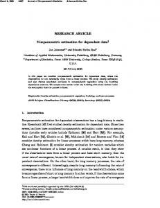
Mar 9, 2009 - 14:57. Journal of Nonparametric Statistics. Johannes-Subba-Rao. RESEARCH ARTICLE. Nonparametric estimation for dependent dataâ .
KEY WORDS: Population pharmacokinetics; nonlinear mixed effects models; density es- timation; nonparametric estimation, maximum likelihood, quinidine. o ...
become more pertinent in light of the large amounts of data that we ...... Along with the development of richer represen
Jun 28, 2012 - Efficient algorithms for fast integration on large data sets from multiple sources .... Several software and packages have also been developed to solve this ...... To achieve a good accuracy, a good threshold value to cut the ...
Fast Construction of a WordâNumber Index for Large Data. MiloÅ¡ Jakub´ıcek, Pavel Rychlý, Pavel Å merk. Natural Lan
number to word indices for very large corpus data (tens of billions of tokens), which is ... database management system
the table from the paper have revealed to be unfair to encodevert. ⢠local data on local hdd, but probably more used.
Fast Algorithms for Generating Delaunay. Interpolation Elements for Domain Decomposition. Philip L. Bowers. Department of Mathematics 3027. Florida State ...
Jul 14, 2016 - We study the fixed design segmented regression problem: Given noisy samples from a ...... Fast, provable algorithms for isotonic regression in.
Feb 1, 1992 - A wide variety of problems can be expressed as fractional packing problems. ..... Ax 5 Xb. We shall use the notation (x, A) to denote that X is the minimum value corresponding to x. ... Hence, X 2 (1 - 3d-1c&d/(ytb) 5 (1 - 3+9* 5 (1 + 6
The columns of ˜Q(2) then form an orthonormal basis ...... 780–804. [23] G. Golub and C. van Loan, Matrix Computations, 3rd ed., The Johns Hopkins University.
We propose and analyze a series of synchrosqueezed transforms (SSTs) to tackle .... One famous method is the empirical mode decomposition (EMD) method ...... G22. 0. Crystal Orientation. Difference in principal stretches. Volume Distortion.
Fast Algorithms for Nonparametric Population Modeling of Large Data ...
May 29, 2008 - curves from large data sets collected in standardized experiments, i.e. with a fixed sampling schedule. It is shown that the overall scheme.
Fast Algorithms for Nonparametric Population Modeling of Large Data Sets Gianluigi Pillonetto a , Giuseppe De Nicolao b , Marco Chierici a , Claudio Cobelli a a Dipartimento
di Ingegneria dell’Informazione, University of Padova, Italy
b Dipartimento
di Informatica e Sistemistica, University of Pavia, Italy
Abstract Population models are widely applied in biomedical data analysis since they characterize both the average and individual responses of a population of subjects. In absence of a reliable mechanistic model, one can resort to the Bayesian nonparametric approach that models the individual curves as Gaussian processes. This paper develops an efficient computational scheme for estimating the average and individual curves from large data sets collected in standardized experiments, i.e. with a fixed sampling schedule. It is shown that the overall scheme exhibits a “client-server” architecture. The server is in charge of handling and processing the collective data base of past experiments. The clients ask the server for the information needed to reconstruct the individual curve in a single new experiment. This architecture allows the clients to take advantage of the overall data set without violating possible privacy and confidentiality constraints and with negligible computational effort. Key words: Nonparametric identification; Bayesian estimation; glucose metabolism; Gaussian processes; estimation theory
1
Introduction
One of the most interesting identification problems arising in biomedical data analysis is the characterization of a population of subjects. Classical examples are found in pharmacokinetics (PK) and pharmacodynamics (PD), where multiple subjects are sampled in order to obtain both the average and individual response to the administered drug. If a sufficiently large number of samples are collected in each individual, it is possible to identify a distinct model for each subject. The typical response of the population could then be obtained from the distribution of the individual models. However, the specific nature of biomedical experiments often poses technological, cost or ethical constraints that permits to collect only few data in each single subject. When the separate identification of individual models is not viable, an effective solution is provided by so-called population modeling approaches [1], [2], [3]. Such methods process all the data simultaneously in order to achieve both the typical and individual models. Although originated in the PK/PD field, population modeling is becoming more and more popular ? Corresponding author Gianluigi Pillonetto Ph. +390498277607 Email addresses: [email protected] (Gianluigi Pillonetto), [email protected] (Giuseppe De Nicolao), [email protected] (Marco Chierici), [email protected] (Claudio Cobelli).
Preprint submitted to Automatica
also in other scenarios as metabolic systems, medical imaging and even genomics [4], [5], [6]. The standard population model is a continuous-time dynamical system containing a finite number of unknown parameters, typically a compartmental model [7]. This leads to a nonlinear-in-parameter identification problem that can be tackled resorting to various iterative algorithms. Among them, one may mention the celebrated NONMEM software [8], which relies on maximum likelihood estimation, but also Bayesian algorithms that compute the posterior distribution of parameters exploiting the Markov chain Monte Carlo (MCMC) machinery [9], [10]. At the early stages of a study or when the mechanistic model of a physiological phenomenon is not available, it may be difficult to formulate a reliable parametric model. Hence the need for flexible nonparametric population approaches that reduce the structural assumptions to a minimum [11]. Along this direction, an example is provided by so-called semiparametric methods that model the response curves as regression splines [12], [13]. A potential difficulty underlying the use of these techniques is the optimization of the number and location of the knots of regression splines, which could suffer from the presence of local minima. More recently, in order to develop a fully nonparametric approach, within a Bayesian paradigm it has been proposed to model the individual curves as realizations of discrete- or continuous-time stochastic processes, e.g. random walks or integrated Wiener
29 May 2008
processes [14], [15]. In these works, each individual curve is seen as the sum of an average curve (common to all subjects) and an individual shift (varying from subject to subject). In particular, both the average curve and the individual shifts are assumed to be Gaussian processes whose statistics are specified by few hyper-parameters. For instance, if the curve is an integrated Wiener process, the hyperparameter is the corresponding intensity. Hyperparameter tuning can be carried out via likelihood maximization. For a given choice of the hyperparameters, the posterior expectations of the processes given the data provide point estimates of the average and individual curves. In particular, when the prior is formulated in terms of integrated Wiener processes, the estimated curves are cubic splines [15]. This Bayesian nonparametric approach has strong connections with kernel methods, Gaussian processes estimation, regularization networks [16],[17]. Recently, a Bayesian MCMC approach able to return the full posterior of hyperparameters and unknown functions has been also worked out, see [18]. In this paper, attention is focused on the nonparametric population analysis of standardized experiments which involve a large number of subjects. Herein, the term standardized is used to denote an experiment that is repeated in multiple subjects adopting a standard sampling schedule. A notable example, treated later in the paper, is the intravenous glucose tolerance test (IVGTT), where glucose plasma concentration is measured after intravenous administration of a glucose bolus. This test is widely employed in the diagnosis of metabolic disorders, see e.g. [19]. In the Bayesian nonparametric approach the computation of the posterior expectations calls for the solution of an algebraic linear system of order nT , where nT is the total number of observations. This is a potential drawback because the complexity scales with the cube of nT . The burden may seem even worse in the case of standardized experiments involving a large number of subjects. As a matter of fact, in the present paper it is shown that the fixed sampling schedule can be exploited to design an algorithm whose complexity scales with the cube of the number of samples collected in each individual. This holds for evaluation of both the posterior expectations and confidence intervals. The new algorithms pave the way to the implementation of a client-server architecture for managing the identification of population models for standardized experiments. The server computes and stores the sufficient statistics abstracted from a large historical data set. The client, whose aim is analyzing a single new experiment (not necessarily standardized), interrogates the server to get the information needed to compute the posterior expectation of the individual curve given all the historical data. The client can also send its data to the server in order to update the centralized sufficient statistics. As an example, the server could be managed by a reference research center, whereas the clients could be laboratories collecting and processing clinical data. According to this architecture, the local laboratories benefit from the information contained in the collective database in a computationally efficient way and without accessing individual data subject to privacy and confidentiality constraints. To the authors’ knowledge, the client-server architecture is a novel
contribution of this paper. In fact, most population modeling approaches cannot be decentralized because of their intrinsic nonlinear-in-parameter structure. The paper is organized as follows. In Section 2 the problem is given its mathematical formulation. In Section 3 the computational algorithms are derived. In Section 4 the proposed methodology is tested on a large data set of IVGTT experiments. Some conclusions end the paper. 2
Statement of the problem
In the sequel, E[.] is used to denote the expectation operator and vectors are column vectors, unless otherwise specified. Further, given two random vectors q and w, let cov[q, w] = E[(q − E[q])(w − E[w])T ] and Var[q] = E[(q − E[q])(q − E[q])T ]. We consider the problem of estimating realizations of continuous-time stochastic processes x j (t), j = 1, 2, . . . , m + 1, from a finite number of noisy samples. The curves x j (t) represent the responses of m + 1 subjects randomly drawn from a population. It is assumed that number and location of the sampling instants do not vary from subject to subject except for what concerns the last one. To be more specific, for j = 1, . . . , m the curves are sampled at instants {tk }, k = 1, 2, . . . , n, while the (m + 1)-th curve is sampled at instants {tk∗ }, k = 1, 2, . . . , n∗ . The measurement model is ykj = x j (tk ) + νkj , ym+1 k
=x
m+1
k = 1, . . . , n,
(tk∗ ) + νkm+1 ,
j = 1, . . . , m ∗
k = 1, . . . , n
where {ν j } = [ν1j . . . νnj ]T , j = 1, . . . , m, and {ν m+1 } = [ν1m+1 . . . νnm+1 ]T are Gaussian and independent random ∗ vectors such that for every k and j E[νkj ] = 0,
Var[ν j ] = Σνj
We assume that the individual curves can be decomposed as x j (t) = x(t) ¯ + xej (t),
j = 1, . . . , m + 1
where x(t) ¯ and xej (t) are zero-mean normal stochastic processes that represent the average curve and the individual shift from the average, respectively. We also assume that processes {νkj }m+1 ¯ and {e x j (t)}m+1 j=1 , x(t) j=1 are all mutually independent. For the sake of simplicity, it is assumed that {e x j (t)}m+1 j=1 are identically distributed. Define now y j = [y1j m+1
y
y2j
= [ym+1 1 £ 1 T
...
ynj ]T ,
ym+1 ... 2 ¤ m T T
y = (y ) . . . (y )
j = 1, 2, . . . , m T ym+1 n∗ ] +
£ y = yT
(ym+1 )T
¤T
The paper is concerned with the solution of the following two estimation problems.
2
• Given y, for any t compute efficiently the continuoustime minimum variance estimate of the average curve x(t), ¯ i.e. E[x(t)|y], ¯ as well as the variance of the reconstruction error, i.e. Var[x(t)|y]. ¯
Proposition 2 Let Reiν = Re + Σiν ,
m
F = ∑ (Reiν )−1 , i=1
m
f = ∑ (Reiν )−1 yi
• Assuming that a new data set ym+1 is available, for any t compute efficiently E[xm+1 (t)|y+ ] and Var[xm+1 (t)|y+ ].
Then,
3
£ ¤−1 T Rˆ ττ = R¯ ττ − R¯ τ F R¯ Tτ + R¯ τ F R¯ −1 + F F R¯ τ E[x( ¯ τ )|y] = r¯τ c
3.1
Computational algorithms
£ ¤ where c ∈ ℜn is given by c = In − F(R¯ −1 + F)−1 f .
Computing E[x(t)|y] ¯ and Var[x(t)|y] ¯
Proof: In view of (4) and (5), we can rewrite Var[y] as follows
The aim is to derive efficient algorithms to compute the estimates E[x( ¯ τ )|y], E[xm+1 (τ )|y+ ], where τ is a generic temporal instant, together with their confidence intervals. We start by introducing the following notation x¯ = [x(t ¯ 1 ) . . . x(t ¯ n )]T x¯τ = [x( ¯ τ ) x(t ¯ 1 ) . . . x(t ¯ n )]T j j j T xe = [e x (t1 ) . . . xe (tn )] , j = 1, 2, . . . , m
(5)
i=1
h 1 i h 1 i 1 T 1 Var[y] = R¯ 2 . . . R¯ 2 R¯ 2 . . . R¯ 2 + bd{Re1ν , . . . , Rem ν}
(1) The matrix inversion lemma (e.g., see page 138 in [20])
Notice that in (2), due to the standardized sampling assumption, Re = Var[e x j ] is independent of j. In the sequel, bd{A1 , . . . , A p } denotes the square block matrix whose diagonal elements are the square matrices A1 , . . . , A p and the off-diagonal elements are zero. We also use Id to denote the d × d identity matrix. The following proposition exploits well known formulas regarding joint Gaussian vectors, see e.g. [20], [21].
Proposition 1 Assuming that the autocovariances of x(t) ¯ and {e x j (t)}m+1 are perfectly known, under the independence j=1 assumptions stated in Section 2, it holds that
−1 } Var[y]−1 = bd{ (Re1ν )−1 , . . . , (Rem (6) ν) (Re1ν )−1 i £ −1 ¤ h .. R¯ + F −1 (Re1 )−1 . . . (Rem )−1 − . ν ν −1 m e (Rν )
(3)
(4)
Further, since x(t), ¯ {e x j (t)} and {ν j } are mutually independent, and the sampling schedule does not vary in the first m subjects, we have that
In view of the above formulas, it would seem that the computation of E[x( ¯ τ )|y] and Rˆ ττ calls for the inversion of an nm-th order matrix. The next proposition exploits the special structure of the problem to demonstrate that only n-th order inverses are required.
Using (3), simple computations provide now the final expression for Rˆ ττ . As regards E[x( ¯ τ )|y], we have that
The last result allows one to compute the estimate of the average curve on an arbitrary sampling grid as well as confidence intervals thanks to the covariance matrix Rˆ ∗ττ . Notice that the formulas require only knowledge of the standardized sampling grid {tk }, necessary in order to compute R¯ τ∗ and R¯ ∗ττ , of matrix F and vector c. In some sense, F and c can be thought of as a sufficient statistic for average curve evaluation, given all the m subjects. In fact, once F and c are known, the individual data {y j }mj=1 are no more necessary. It is now shown how to efficiently compute E[xm+1 (τ )|y+ ] as a function of E[x¯τ∗ |y] and Rˆ ∗ττ . To obtain this goal, it is use∗ and E[x¯∗ |y] into submatrices as follows: ful to partition Rˆ ττ τ
h i E[x( ¯ τ )|y] = cov[x( ¯ τ ), y1 ] . . . cov[x( ¯ τ ), ym ] Var[y]−1 y Using (6),
¡ ¢T Var[y]−1 y = c1 . . . cm
(7)
where "
¡ ¢−1 m j −1 j ci = (Reiν )−1 yi − (Reiν )−1 R¯ −1 + F ∑ (Reν ) y
In the previous subsection, a method has been obtained to efficiently compute the estimate of the average curve of the population from data collected in m subjects on a standardized grid {tk }. Assume now that such data are already available and that a new (m + 1)-th subject is sampled on an arbitrary sampling grid {tk∗ }. In this subsection, we show how to estimate the individual curve of the new subject taking into account all the available information on the previous m subjects. We start by reporting a notation which refers to the sampling grid {tk∗ }. and which represents an extension of that reported in (1) and (2). Let
Proof To obtain the results, one can first replace ym+1 with x¯∗ + xem+1 + ν m+1 and xm+1 (τ ) with x( ¯ τ ) + xem+1 (τ ). After ∗ m+1 that, one exploits the fact that x¯ , xe and ν m+1 are indem+1 pendent of each other and that xe and ν m+1 are independent of y. 2 We are now in a position to compute E[xm+1 (τ )|y+ ] and the variance of the error affecting such estimate as a function of the submatrices of Rˆ ∗ττ and E[x¯τ∗ |y] given in (8). The following proposition exploits well known results on joint Gaussian vectors (e.g., see [20, Section 3.1]) and Lemma 4.
Proposition 5 It holds that rτ∗ }(P + Re∗ + Σm+1 )−1 E[xm+1 (τ )|y+ ] = ξτ + { p¯ + e ν × (ym+1 − ξ ) m+1 + Var[x (τ )|y ] = p + e rτ − { p¯ + e rτ∗ } × (P + Re∗ + Σm+1 )−1 { p¯ + e rτ∗ }T ν
The next proposition (whose proof is omitted) shows how to calculate efficiently Rˆ ∗ττ and E[x¯τ∗ |y]. Proposition 3 Consider quantities Reiν , F and c as defined in Proposition 2. Then,
The last result shows that the estimate of the (m + 1)-th individual curve depends only on the corresponding data ym+1 and matrix Rˆ ∗ττ and vector E[x¯τ∗ |y] in (8), which summarize all the information from the other m subjects. Recall that Rˆ ∗ττ
and E[x¯τ∗ |y] depend only on F and c. Thus, one can imagine a distributed estimation scheme based on the following client-server architecture. The server processes m subjects sampled on a standardized grid {tk } and calculates matrix F and vector c. The client processes the data of the (m + 1)-th subject as follows: it asks the server for F and c and then uses them to obtain the individual curve. In this way, the client is able to exploit the whole data set made of m subjects without having access to the data. Finally, notice also that, if we suppose that the (m + 1)-th subject has a standard sampling schedule, then its data can be sent to the server in order to update F and c. This will allow other clients to benefit from the information contained in ym+1 . It is worth stressing that such update operation can be performed very efficiently. In fact, denote with F u and cu the updated versions of F and c, respectively. Then, exploiting the results reported in Proposition 2, the following update formulas easily follow
f =f
Proposition 7 The determinant of the nm × nm matrix Var[y] can be computed as à det(Var[y]) =
!2
∏ det(Cii )
where Cii are n × n matrices such that Cii = chol[Aii − Di ],
C(i+1)i = (R¯ − Di ) (CiiT )−1
Cki = C(i+1)i for k > i + 1,
T Di+1 = Di +C(i+1)iC(i+1)i
T )−1 . ¯ 11 with the initial positions D1 = 0 and C21 = R(C
)−1 ym+1 + (Rem+1 ν 4
3.3
m
i=1
h ¡ ¢−1 i u cu = In − F u R¯ −1 + F u f
F u = F + (Rem+1 )−1 ν u
In the sequel, we use chol[K] to denote the Cholesky factorization of the matrix K [20]. Let also Akk = R¯ + Re + Σkν indicate the k-th n × n block on the diagonal of Var[y]. The second result (whose proof is omitted) is reported below.
Example
Computing unknown hyper-parameters In this Section, the proposed computational scheme is tested on a database that consists of 224 healthy subjects, on which an intravenous glucose tolerance test (IVGTT) was performed. The first 204 subjects represent our training set. It consists of standardized experiments where the same sampling schedule was adopted for all subjects and plasma glucose samples were collected non-uniformly between 0 and 240 min [22]. To be specific, n = 20 and the set Ω1 , expressed in minutes, corresponds to the sampling instants {tk } given by {2, 4, 6, 8, 10, 15, 20, 22, 25, 26, 28, 31, 35, 45, 60, 75, 90, 120, 180, 240}. Data regarding the remaining 20 subjects are selected from IVGTT studies described in [5,23,24], in which a glucose dose, identical to that administered in the first 204 subjects, was injected at time zero. In particular, in the first 13 subjects n = 30 and the sampling grid, denoted by Ω1 and expressed in minutes, is {2, 3, 4, 5, 6, 8, 10, 12, 15, 20, 22, 24, 26, 28, 30, 35, 40, 45, 50, 55, 60, 70, 80, 100, 120, 140, 160, 180, 210, 240}. In the last 7 subjects n = 29 and the sampling grid, denoted by Ω2 , is {2, 3, 4, 5, 8, 10, 12, 14, 16, 18, 20, 24, 28, 32, 40, 45, 50, 60, 70, 80, 90, 100, 110, 120, 140, 160, 180, 210, 240}. In all the 224 subjects, measurements are known to be corrupted by a white normal noise with a 2% coefficient of variation. Glucose data were pre-processed by first subtracting the basal value from each profile. To take into account the fact that processed glucose data tend to zero, a time transformation of t was performed so that the new time e t ranges from 0 to 1, according to the formula e t = 1/(1 + t/γ ), as in [15]. We set parameter γ to 30, a value that maximizes the minimum distance between each pair of transformed sampling instants given by the union of the sampling grids associated with the 224 subjects. Both the typical curve and the individual shifts were modelled as integrated Wiener processes.
When dealing with real world problems, the autocovariances of the signals of interest may contain unknown hyperparameters which have to be estimated from data. To tackle this problem, we resort to the so-called Empirical Bayes method where a Maximum Likelihood (ML) estimate of hyper-parameters is first achieved. Next, parameters are set to their ML estimates and the Bayes estimate is computed using the formulas described in the previous sub-sections. Within the client-server architecture outlined at the end of the previous subsection, it is the server that is in charge of estimating the hyperparameters and transmitting them to the clients. In fact, the client needs the hyperparameters in order to be able to evaluate the autocovariances which enter the computational formulas. Now, assume that the unknown hyper-parameters are contained in the parameter vector θ that parametrizes Var[y]. To compute their estimates, the following optimization problem has to be solved
θˆ = arg min J(y; θ ) θ
where J(y; θ ) = log[det(Var[y])] + yT Var[y]−1 y is equal to the opposite of the log-likelihood apart from a constant. In the following two propositions, it is shown that evaluation of the log-likelihood for a given θ requires only O(m × n3 ) operations. The first result can be immediately deduced by exploiting (7). Proposition 6 It holds that yT Var[y]−1 y = yT c
5
Population (reduced sampling)
50
0
50
0
0
60
120
180
−50
240
0
60
min
Single−subject (full sampling)
120
180
Population (reduced sampling)
140
140
120
120
100
100
80
80
−1
mg dl−1
100
mg dl−1
mg dl−1
100
−50
Population (full sampling)
150
60
mg dl
Population (full sampling) 150
40 20
60 40 20
0
0
−20
−20
−40
−40
240
0
60
120
180
min
min
Single−subject (reduced sampling)
Single−subject (full sampling)
240
0
60
120
180
240
min
Single−subject (reduced sampling)
150
150
100 100
100
50
50 0
mg dl−1
50
mg dl−1
mg dl−1
mg dl−1
100 50
0
−100
−50
0
0 −50
−50
−150
−100 −50
0
60
120
180
240
0
60
min
120
180
240
0
60
min
120
50
0
−50
50
0
0
60
120
180
−50
240
140
140
120
120
100
100
−1
160
80 60 40 20
0
60
min
120
180
240
40 20 0
−20
−20 0
60
120
180
240
0
60
50
140
140
120
120
100
100
−1
160
80 60 40 20
0
0
−50
−50
0
60
120
180
240
0
60
min
120
180
240
240
80 60 40 20
0
0
−20
−20 0
min
60
120
180
240
0
min
(c) Subject #215
180
Single−subject (reduced sampling)
160
mg dl
50
100
mg dl−1
mg dl−1
mg dl−1
150
120
min
Single−subject (full sampling)
Single−subject (reduced sampling)
100
240
60
min
150
180
80
0
min
Single−subject (full sampling)
120
Population (reduced sampling)
160
mg dl
100
60
min
Population (full sampling)
mg dl−1
100
0
(b) Subject #214 Population (reduced sampling)
150
mg dl−1
mg dl−1
Population (full sampling)
−200
240
min
(a) Subject #209
150
180
60
120
180
240
min
(d) Subject #219
Fig. 2. Estimation of individual IVGTT responses. Comparison between Population approach and Single-subject approach in 4 representative subjects. The Population approach exploits information from other 204 IVGTT experiments.
As previously observed, hyperparameters λ¯ and e λ have to be estimated from data. Data relative to the first m = 204 subjects were exploited to estimate hyper-parameters via maximum likelihood. One can think of the computations related to such data base as e.g. performed by a reference research center which has access to a large data set. Obtained values for λ¯ and e λ turned out to be around 13700 and 4440, respectively. After that, each of the remaining 20 “(m + 1)-th” curves, was estimated by applying the method discussed in Section 3, hereby called “population approach”. For comparison, the “(m + 1)-th” profiles were also estimated without exploiting information regarding the first 204 subjects. In particular, curves were modeled as integrated Wiener processes with regularization parameter estimated via maximum likelihood and adopting the same time transformation e t . Note that, under the integrated Wiener prior, the estimated curves are cubic smoothing splines [25]. This approach will be hereby called “single-
200
mg dl−1
150
100
50
0
0
60
120
180
240
min
Fig. 1. Estimated average curve obtained by Population approach applied to 204 IVGTT responses
Thus, it holds that (see also [15]) ( 2¡ ¢ s s 2 2 τ−3 ¯ cov(x(s), ¯ x( ¯ τ )) = λ ¡ ¢ τ2 τ 2 s− 3 ( 2¡ ¢ s s 2 j j 2 τ−3 e cov(e x (s), xe (τ )) = λ ¡ ¢ τ2 τ 2 s− 3
s≤τ s>τ s≤τ s>τ
∀j 6
Population (full sampling)
50
Population (reduced sampling)
45 150
150
100
100
50
0
0
−50
−50 0
60
120
180
35
50
240
Values
−1
mg dl
mg dl−1
40
60
1000
100
500
−1
200
0
−500
−200
−1000
60
120
240
15
180
min
10
240
5 Population
−1500
0
60
120
180
240
sampling grid but not used in the estimation process. Fig. 4 plots boxplots of the 20 computed values of RMSE using the population and single subject approach. It is apparent that the population approach outperforms the single-subject one in terms of predictive capability on new glucose data.
subject approach”. As concerns measurements related to the “(m + 1)-th” subject, we employed both a full and reduced sampling schedule. In the latter, when dealing with the sampling grid Ω1 , n∗ is fixed to 15, and the set {tk∗ } corresponds to {2, 4, 6, 10, 15, 22, 26, 30, 35, 45, 55, 80, 120, 160, 240}. When dealing with the sampling grid Ω2 , n∗ is still 15 but the set {tk∗ } now corresponds to {2, 4, 5, 10, 14, 18, 24, 32, 40, 50, 60, 80, 120, 160, 240}. One can think of computations related to the “(m + 1)-th” curves as performed by clients such as laboratories collecting clinical data. Fig. 1 plots the estimated average curve. The results regarding 4 representative subjects (#209, #214, #215 and #219) are instead visible in Fig.2 where t is used as time axis. In each of the sub-figures, fully sampled data vs. estimated curves are plotted for the population approach (top-left) and the single-subject one (bottom-left). The remaining two panels in each sub-figure show reduced data vs estimated curves for the population approach (top-right) and single-subject one (bottom-right). Rather interestingly, the curves reconstructed via the single-subject approach suffer from oscillations in the final part of the experiment (t > 120 min), where data are sampled less frequently. On the other hand, the population approach is less influenced by the sampling schedule. In fact, good results are obtained with both full and reduced sampling. In Fig. 3 we show results regarding subject #211 reporting estimated curves and ±1SD confidence bands (dashed lines). It is apparent that confidence intervals obtained by the population approach are narrower than those obtained by the single-subject approach. To obtain a global comparison of the two approaches, given the full and reduced sampling grids I f and Ir , respectively, define I = I f Ir . Then, for every “(m + 1)-th” subject we compute the quantity
5
Conclusions
In this paper, efficient formulas have been developed for the nonparametric estimation of population models from large data sets collected in experiments adopting a standardized sampling schedule. In particular, the structure of the problem has been exploited to design algorithms whose complexity scales with the cube of the number of data collected in a single subject, while previous algorithms [15,18] scaled with the cube of the total number of observations. The overall identification scheme presents a “client-server” architecture. The server takes care of managing historical information on past experiments. The client deals with a single new experiment and interrogates the server to obtain the information needed to reconstruct the individual curve. In this way, clients exploit the global data set without having access to the historical data and with negligible computational effort. A data base of 224 IVGTT experiments has been employed to successfully validate the approach. Obtained results show that the individual estimates provided by the population approach are much more satisfactory than those achievable from the single experiment. In addition, when the sampling schedule of a subject is reduced, the individual estimate obtained by the population approach remains satisfactory whereas the quality of the single-subject estimate shows a further degradation. Acknowledgments We thank Dr. R.A. Rizza and Dr. R. Basu (Mayo Clinic, Rochester, MN USA) for having made available to us the IVGTT data of [22]. Data described in [5,23,24] were downloaded from the website of the Resource Facility for Population Kinetics (http://www.rfpk.washington.edu). This research has been partially supported by FIRB Project ”Learning theory and application”, by NIH/NIBIB grant P41-EB01975 and by the PRIN Project ”New Methods
s RMSE =
Single−subject
Fig. 4. Estimation of individual IVGTT responses. Comparison of RMSE obtained by Population approach and Single-subject approach in 20 subjects
0
−100
0
180
Single−subject (reduced sampling)
mg dl
mg dl−1
Single−subject (full sampling)
−300
120
min 1500
25 20
0
min 300
30
ˆ 2 ∑t∈I (ym+1 (t) − x(t)) n − n∗
where x(t) ˆ = E[xm+1 (t)|y+ ]. Notice that the smaller RMSE, the larger the predictive capability at times falling in the full
7
and Algorithms for Identification and Adaptive Control of Technological Systems”.
[20] B. D. O. Anderson and J. B. Moore. Optimal Filtering. PrenticeHall, Englewood Cliffs, N.J., USA, 1979. [21] A. N. Shiryaev. Probability. Springer, New York, NY, USA, 1996.
[1] S. L. Beal and L. B. Sheiner. Estimating population kinetics. Crit. Rev. Biomed. Eng., 8(3):195–222, 1982.
[22] R. Basu, C. Dalla Man, M. Campioni, A. Basu, G. Klee, G. Jenkins, G. Toffolo, C. Cobelli, and R.A. Rizza. Effect of age and sex on postprandial glucose metabolism: difference in glucose turnover, insulin secretion, insulin action, and hepatic insulin extraction. Diabetes, 55:2001–2014, 2006.
[2] L. B. Sheiner. The population approach to pharmacokinetic data analysis: rationale and standard data analysis methods. Drug Metabolism Reviews, 15:153–171, 1994.
[23] P. Vicini, A. Caumo, and C. Cobelli. The hot IVGTT twocompartment minimal model: indexes of glucose effectiveness and insulin sensitivity. Am. J. Physiol., 273:1024–1032, 1997.
[3] M. Davidian and D. M. Giltinan. Nonlinear Models for Repeated Measurement Data. Chapman and Hall, New York, 1995.
[24] P. Vicini, J.J. Zachwieja, K.E. Yarasheski, D.M. Bier, A. Caumo, and C. Cobelli. Glucose production during an IVGTT by deconvolution: validation with the tracer-to-tracee clamp technique. Am. J. Physiol., 276:285–294, 1999.
References
[4] A. Bertoldo, G. Sparacino, and C. Cobelli. “Population” approach improves parameter estimation of kinetic models from dynamic PET data. IEEE Trans. on Medical Imaging, 23(3):297–306, 2004.
[25] G. Wahba. Spline Models for Observational Data. Philadelphia, 1990.
[5] P. Vicini and C. Cobelli. The iterative two-stage population approach to IVGTT minimal modeling: improved precision with reduced sampling. Am. J. Physiol. Endocrinol. Metab., 280(1):179–186, 2001. [6] F. Ferrazzi, P. Magni, and R. Bellazzi. Bayesian clustering of gene expression time series. In Proc. of 3rd Int. Workshop on Bioinformatics for the Management, Analysis and Interpretation of Microarray Data (NETTAB 2003), pages 53–55, 2003. [7] J.A. Jacquez. Compartmental analysis in biology and medicine. Ann Arbor: University of Michigan Press, 1985. [8] S. Beal and L. Sheiner. NONMEM User’s Guide. NONMEM Project Group, University of California, San Francisco, 1992. [9] W.R. Gilks, S. Richardson, and D.J. Spiegelhalter. Markov chain Monte Carlo in Practice. London: Chapman and Hall, 1996. [10] D. J. Lunn, N. Best, A. Thomas, J. C. Wakefield, and D. Spiegelhalter. Bayesian analysis of population PK/PD models: general concepts and software. J. Pharmacokinet. Pharmacodyn., 29(3):271–307, 2002. [11] I.A. Ibragimov and R.Z. Khasminskii. Asymptotic Theory. Springer, 1981.
Statistical Estimation:
[12] K. E. Fattinger and D. Verotta. A nonparametric subjectspecific population method for deconvolution: I. Description, internal validation, and real data examples. J. Pharmacokin. Biopharm., 23:581–610, 1995. [13] K. Park, D. Verotta, T. F. Blaschke, and L. B. Sheiner. A semiparametric method for describing noisy population pharmacokinetic data. J. Pharmacokin. Biopharm., 25:615–642, 1997. [14] P. Magni, R. Bellazzi, G. De Nicolao, I. Poggesi, and M. Rocchetti. Nonparametric AUC estimation in population studies with incomplete sampling: a Bayesian approach. J. Pharmacokin. Pharmacodyn., 29(5/6):445–471, 2002. [15] M. Neve, G. De Nicolao, and L. Marchesi. Nonparametric identification of population models via Gaussian processes. Automatica, 43:1134–1144, 2007. [16] C.E. Rasmussen and C.K.I. Williams. Gaussian Processes for Machine Learning. The MIT Press, 2006. [17] T. Evgeniou, C.A. Micchelli, and M. Pontil. Learning multiple tasks with kernel methods. J. Machine Learning Research, 6:615–637, 2005. [18] M. Neve, G. De Nicolao, and L. Marchesi. Nonparametric identification of population models: An MCMC approach. IEEE Trans. on Biomedical Engineering, 55:41–50, 2008. [19] R.N. Bergman, C.R. Bowden, and C. Cobelli. Carbohydrate Metabolism, chapter The minimal model approach to quantification of factors controlling glucose disposal in man. Wiley, New York, 1981.