Fast free-form deformation using graphics processing units - CiteSeerX

Fast Free-Form Deformation using Graphics Processing Units Marc Modata , Gerard R. Ridgwaya,b , Zeike A. Taylora , Manja Lehmannb , Josephine Barnesb , David J. Hawkesa , Nick C. Foxb , S´ebastien Ourselina,b a

Centre for Medical Image Computing, Department of Medical Physics and Bioengineering, University College London, UK b Dementia Research Centre, Institute of Neurology, University College London, UK

Abstract A large number of algorithms have been developed to perform non-rigid registration and it is a tool commonly used in medical image analysis. The FreeForm Deformation algorithm is a well-established technique, but is extremely time consuming. In this paper we present a parallel-friendly formulation of the algorithm suitable for Graphics Processing Unit execution. Using our approach we perform registration of T1-weighted MR images in less than 1 minute and show the same level of accuracy as a classical serial implementation when performing segmentation propagation. This technology could be of significant utility in time-critical applications such as image-guided interventions, or in the processing of large data sets. Key words: GPU, Non-Rigid Registration, Free-Form Deformation, Normalised Mutual Information

Preprint submitted to Computer Methods and Programs in Biomedicine August 28, 2009

1. Introduction In the field of medical image analysis, image registration remains one of the main research topics and challenges. Image registration consists of deforming a floating image to match a reference image. The most active area of research is non-rigid registration (NRR), in which attempts are made to locally “warp” one image into correspondence with another. Example problems are matching 3D MRI scans of two different patients, or two scans of the same patient before and after surgery. While a huge amount of research has been devoted to the methodological development [1, 2], very little research has focused on the computational burden of the proposed algorithms. One of the most widely used NRR algorithms, Free-Form Deformation [3] (FFD), has not reached its full clinical utility as a result; FFD’s computation time on a single data set can extend to several hours. If such constraints could be removed, or alleviated a new range of clinical applications, which require real-time or near real-time computation could be attempted. Such applications arise, for instance, in the context of real-time image-guided surgery: new patient information acquired during surgery, such as ultra-sound images, could be used efficiently to update a previously developed surgical plan. The bottleneck of the FFD algorithm is the cubic B-Spline computation, and consequently work has been done to speed up this part using various architectures. Jiang et al. [4] used a FPGA-based implementation which lead to a speed-up of 3.2 times compared to a 2.666 GHz CPU execution. Rohlfing et al. [5] reduced computation time by more than 50 times using 64 CPUs of a shared-memory supercomputer. More recently, Rohrer et al. [6] presented a multicore implementation of the B-Spline computation based 2

on a Cell Broadband EngineT M (Cell/B.E.) platform. Their architecture performed 40% faster than serial execution on a standard computer. These techniques provide considerable computation time improvements, however they require either high technical knowledge or hardware with prices inhibiting wide adoption. We propose the use of graphics processing units (GPUs) as a cost effective high performance solution. Moreover we advocate use of NVidia Corporation’s CUDA API, which requires only knowledge of the C language and very little awareness of the hardware. In this article we present a data parallel formulation of the FFD algorithm and describe its execution on GPU architecture using the CUDA API. The formulation affords particularly efficient memory use, allowing much improved use of computational resources. The resulting system provides significant speed improvements, without resorting to theoretical or numerical approximations. In the first section we present the methodology and its GPU-based implementation. In the second we present the computation time benefit from such an implementation, and evaluate the formulation’s accuracy. The time benefit is simply assessed by comparing the computation time of a serial and a parallel implementation of the same algorithm. The accuracy is evaluated by comparing the result of segmentation propagation using our GPU implementation and the classical serial FFD formulation.

3

2. Method 2.1. The Free-Form Deformation algorithm The main requirement for an algorithm to benefit from GPU execution is data parallelism. The FFD algorithm comprises three components, which may be considered independently: transformation of the floating image using the splines and an interpolation function; evaluation of an objective function; and optimisation against this function. Individually, these components may be formulated in a data parallel manner as they mainly consist of voxel-wise computations. However difficulties associated with GPU memory constraints mean certain aspects are not easily implemented in practice. 2.1.1. Cubic B-Splines interpolation The FFD algorithm consists of locally deforming an image volume using cubic B-Splines. This technique has the desirable feature of guaranteeing a C 2 continuous deformation (see Fig. 1). The cubic B-Splines framework is well documented elsewhere [3], and the details are omitted for brevity. However we note that a particularly favourable property of the framework is that any deformation produced with a grid of density n can be exactly produced on a grid of density 2n − 1. This property has been used in a pyramidal approach in our implementation. However, cubic B-Spline methods are extremely computationally expensive. For this reason in the classical approach only one control point is optimised at a time, which means the whole image does not have to be fully interpolated at each step. The computation of each voxel’s position and their new intensities are fully independent and thus their computation is suitable 4

for parallel implementation. Since GPU-based computation is more efficient when processing large amounts of data concurrently, we optimise all control points and interpolate the whole image at each step. The deformation T which optimises an objective function between the deformed floating image F (T) and the reference R is sought. 2.1.2. Metric computation The Normalised Mutual Information (NMI) is a voxel intensity-based information-theoretic similarity measure based on the paired-intensity distribution in R and F(T). A larger NMI value reflects a greater level of shared information between the two images. It is computed from NMI =

H(R) + H(F (T)) , H(R, F (T))

where H(R), H(F (T)) and H(R, F (T)) are respectively the two marginal entropies and the joint entropy. Its computation thus requires a joint histogram which, in our implementation, was filled using a Parzen Window (PW) approach[7]. In order to promote smooth deformation, a penalty term P has been added to the NMI value. The objective function C to be optimised is a balance between the NMI similarity measure and the deformation penalty: C = (1 − α) × NMI − α × P,

(1)

where 0 ≤ α < 1. The penalty-term we describe here, the bending-energy,

5

was used for non-rigid registration by Rueckert et al.[3]. It is defined as  2  2 2  2 2 1 X ∂ 2 T(~x) ∂ T(~x) ∂ T(~x) P = + + N ∂x2 ∂y 2 ∂z 2 ~ x∈Ω " 2  2 2  2 2 # ∂ T(~x) ∂ T(~x) ∂ 2 T(~x) + + , (2) + 2× ∂xy ∂yz ∂xz where N is the voxel number in Ω, the domain of R. We approximated this penalty term by computing the bending-energy values at the control point positions only, which reduced the number of computations. Furthermore, as explained in Rohlfing et al.[5], this approach allowed precomputation of the cubic B-spline basis values for each node, thus easing the calculation further. 2.1.3. Control point position optimisation To optimise the control point positions, we used a conjugate gradient ascent. This approach is more efficient than a simpler steepest ascent optimisation, and is less memory intensive than Newton type algorithms. We thus required the derivative ∂ C of the objective function: ∂µξijk

∂C ∂µξijk

= (1 − α) ×

∂NMI ∂µξijk

−α×

∂P ∂µξijk

,

(3)

where ξ are the x, y and z components of the control point µijk . The gradient of the NMI is calculated as: ∂NMI ∂µξijk

=

∂H(R) ∂µξijk

+

∂F (T) ∂µξijk

− NMI ×

H(R, F (T))

∂H(R,F (T)) ∂µξijk

,

which requires computation of the derivative of the marginal and joint entropies. These can be computed from the derivative of the intensity distribution, which requires the derivative of the joint histogram H[8]: ∂βf3 (i, f ) ∂H(r, f ) X 3 ∂F (p) ∂T(~x) = β (R(~ x ); r) r ξ ∂i ∂p p=T(~x) ∂µξijk ∂µijk i=F (T(~ x)) ~ x∈Ω 6

(4)

This approach provides the mathematical value of the gradient but involves significant computational redundancy, since each voxel is included in the neighborhood of several control points. Moreover it is memory intensive as each node requires one joint histogram per degree of freedom. In order to decrease this redundancy and the memory requirement, we propose a voxelcentric approach to evaluate the node-centric gradient. We first compute the gradient value for every voxel, then gather the information from all voxels to obtain the nodal gradient values. ∂H(r,f ) using the formulas ∂uξz where ∂T(x) = I if z = x as ∂uξz

We computed the voxel-centric gradient values in equation 4, with

∂T(x) ∂µijk

replaced by

∂T(x) , ∂uξz

T(x) = x + u(x). From the voxel-centric gradient values, we extracted the analytical nodecentric derivative of the similarity measure. We first applied a convolution window to the gradient field where the convolution window was a cubic BSpline curve which matched the basis functions in the deformation model in terms of node spacing; it was equivalent to

∂T(x) ∂µijk

in equation 4. Secondly, we

extracted the gradient value from the smoothed image at the node position. As seen in equation 3, the gradient of the bending energy is required also. P Abbreviating equation 2 as P = N1 ~x∈Ω A2 + B 2 + C 2 + 2D 2 + 2E 2 + 2F 2 , the derivative of the penalty term involves a sum of derivatives each of which ∂ (A 2 ) ∂ (A 2 ) can be obtained using the chain rule, e.g. ∂µξ = ∂A . ∂µ∂A = 2A ∂µ∂A ξ ξ . As ijk

ijk

ijk

for the bending energy evaluation, and for the same reason, this gradient was computed at the control point positions only.

7

2.2. A GPU-based implementation The F3D implementation was achieved using CUDA [9] which is an Application Programming Interface developed by NVidia to simplify the interface between CPU (host) and GPU (device). Our framework comprises four steps, organised as in Fig. 2. The first step performs image interpolation via cubic B-Splines and trilinear interpolation to define the new voxel position and intensity. As already stated the computation of each voxel’s displacement and intensity interpolation is independent and their parallel hardware implementation is therefore straightforward. However the calculations are demanding in terms of dynamic memory resources, requiring allocation of around 22 registers per computational thread. As GPU memory is limited, a higher register requirement per thread dictates that fewer threads may be executed concurrently, resulting in sub-optimal use of the device’s computational resources. The ratio of active threads to maximum allowed (hardware dependent) is referred to as occupancy [9], and an efficient implementation should maximise this. A single kernel requiring 22 registers leads to an occupancy of 42%. For this reason this step has been split into two kernels, the first dealing with the B-Splines interpolation only and the second with trilinear interpolation. Register requirements then fall to 16 and 12 respectively, and occupancies increase to 67% and 83%. Such a technique allows a computation time improvement of 36.8% in our case. The second step involves filling the whole joint histogram and computing the different entropy values. A GPU implementation of this step did not show a significant reduction in computation time compared with serial im8

plementation. Furthermore this step occupies only around 2.2% of the entire computation time. Moreover a GPU implementation necessitates use of single precision which, for this step, proves detrimental to accuracy1 . For these reasons this step is executed on CPU rather than on GPU. This choice does not affect the computation time even with the data transfer between device and host. In the third step the gradient value is computed for each voxel and the convolution windows are applied. As for the first step, we distributed the computation across several kernels to improve occupancy. The first kernel computed the gradient values. The gradient was then smoothed using three different kernels, each dealing with one axis. For these kernels it appeared that computing the cubic spline curve “on the fly” was faster than precomputing and fetching them from memory. The last step normalises the gradient and updates the control point positions using a conjugate gradient optimisation. A first kernel is used to extract the maximal gradient value from the whole field. The field is split into several parts from which a maximal value is extracted. Subsequently, the largest value from the extracted maximas is kept. A last kernel updates the control point positions based on the normalised gradient value. A final feature of our approach is the use of a convergence criterion. Whereas time constraints dictated that earlier implementations [3] performed a set (and small) number of iterations, our algorithm iterates until convergence, aiming to ensure better registration. 1

Newer devices do offer double precision accurary, but at a significant lower

performance[9]

9

We used an NVidia 8800GTX GPU, which included 128 processors and 768 MB of memory. The memory size was a limitation as it prohibited loading very large image sets with a small control point spacing δ. Nonetheless we managed to run tests on 2563 voxel images with δ = 2.5 voxels along each axis. These specifications are generally acceptable for MR brain images for example. Moreover, recently released card have an increase amount of memory, up to 4 GB for example2 . 3. Evaluation 3.1. Computation time evaluation To evaluate the benefit of a GPU-based implementation, our parallelfriendly algorithm has been implemented in both C++ and CUDA. The speed improvements presented in Table 1 were obtained using a 3.0GHz CPU and an NVidia 8800 GTX GPU. The image sizes were 181×217×181 voxels and the spline lattice contained 40×44×40 control points, which is common for inter-subject brain MR images. The overall speed improvement from the GPU implementation was 9.89 times. This value includes the data transfer between host and devices, as well as the registration initialisation. For this reason, 9.89 does not correspond to the mean of the speed improvements for each function in Table 1. A non-rigid registration using the FFD approach (see Fig. 3) was performed in 42 sec on standard T1 weighted MR brain images. 2

www.nvidia.com/page/hpc.htm

10

Function

Speed improvement

Deformation field computation

× 11.27

Trilinear resampling

× 12.83

Cubic spline resampling

× 10.12

Bending-energy computation

× 9.13

NMI gradient computation

× 26.30

Bending-energy gradient computation

× 13.33

Table 1: Speed improvements of parallel GPU computation over serial CPU computation for each function in the implementation.

3.2. Registration accuracy evaluation In order to assess the accuracy of our implementation we performed segmentation propagations and compared the results with those obtained from a classical FFD implementation3 . The dataset consisted in 20 T1weighted brain MR images, of which 10 scans were of clinically-diagnosed Alzheimer’s disease (AD) patients and 10 age-matched control subjects. The data acquisition protocol as well as the subject characteristics have been described by Chan et al. [10]. The size of the images used in the registration was 180 × 180 × 124 voxels, with a voxel spatial resolution of 0.9375 × 0.9375 × 1.5mm3 . For each brain image, different manual segmentations have been performed. The regions of interest are listed in table 2 and a few are illustrated in figure 4. 3

A FFD algorithm executable can be downloaded from Daniel Rueckert’s webpage:

http://www.doc.ic.ac.uk/∼dr

11

Using our Fast-FFD and the classical serial FFD, we performed 380 (20 × 19) registrations in which each scan was registered to all others. As scans of both diagnosed AD patients and controls were used, we expected significantly differing brain shapes and correspondingly significant deformations to be recovered by the algorithms. Prior to the non-rigid registration, an affine registration has been performed using FLIRT [11]. All the non-rigid registrations were performed with a pyramidal approach with 3 levels. The finer lattice of control points had a spacing of 5 mm along each axis. Both algorithms employed a conjugate gradient optimisation, and a bending energy weight of α = 1% (Eq. 1). As a preprocessing step, each T1w MR image was skull stripped using BET [12] and a dilation was applied on the obtained mask. The resulting set of deformation fields were then used to propagate the manually segmented masks between images. We computed the Dice similarity (DS), as in equation 5, between each manual segmentation (Mm ) and the corresponding propagated (Mp ) region of interest. DS = 2 ×

||Mm ∩ Mp || ||Mm || + ||Mp ||

(5)

The DS rates the overlap of two masks between 0 and 1, where 1 indicates a perfect overlap and 0 none. Table 2 summarizes the obtained results using both implementations. For comparison, the DS was computed using only an affine transformation also. For these data the mean registration time was around 5 hours per image using the classical FFD algorithm, but less than 20 seconds using our GPUbased implementation. For comparison, our implementation had a mean computation time of 3 minutes 18 seconds when running on the same CPU.

12

3.3. Discussion The comparison of our CPU and GPU implementations of the presented algorithm (section 3.1) showed a speed-up of approximately 10 times using the latter. We conclude that the algorithm maps well to parallel architectures, and consequently is well-suited to GPU execution. However, for the segmentation propagation examples (section 3.2) dramatically higher performance was shown by our formulation (and implementation) compared with the classical algorithm. Thus the majority of the speed improvement arises from the improved formulation, rather than the GPU implementation itself. Two features of the formulation are likely to be responsible: (1) optimisation of all control points concurrently, rather than serially, and (2) use of an analytical objective function gradient, rather than a symmetric difference estimate. The latter, in particular, is significant: a symmetric difference evaluation is time consuming as it requires resampling of the floating image and evaluation of the objective function value six times per control point. Moreover, the use of the analytical metric gradient may lead to a faster conjugate gradient convergence. The DS evaluation showed that both the classical FFD and our implementation improved the overlap between regions of interest, compared to a single affine registration. Moreover the Fast-FFD method appears to perform better in most cases; the higher values are statistically significant for the left and right entorhinal cortex and the left parahippocampal gyru when performing a paired t-test (p < 0.01). The improvements can be attributed to the use of a stopping criteria based on the objective function value (and the consequent increase in the number of iterations performed) in the Fast-FFD method. To limit computation time we used a maximum of 13

10 iterations in the classical FFD. 4. Conclusion Non-rigid registration is a central but computationally-expensive tool in medical imaging. We have developed an efficient data-parallel formulation of the widely used FFD algorithm which maps well to high performance GPU architectures. Our implementation performed the registration in Fig. 3 in less than one minute, making possible the analysis of very large cohorts of subjects, with the aim of better understanding diseases such as Alzheimer’s. By alleviating time constraints the approach could also allow development of new time-critical application areas, for example in surgical planning and navigation. Code The GPU-based code which has been used to process the data in the article can be downloaded from http://cmic.cs.ucl.ac.uk/staff/marc modat/code/ Acknowledgments The authors are very grateful to Tristan Clark for his helpful support in order to efficiently use the cluster to run the linear classical FFD. Some of this work was undertaken in University College London Hospitals/University College London, which received a proportion of funding from the UK Department of Health’s National Institute of Health research Biomedical Research Centres funding scheme. N.C. Fox is supported by a Medical Research Council (UK) Senior Clinical Fellowship. J. Barnes is supported by an Alzheimer’s 14

Research Trust (UK) research fellowship with the kind support of the Kirby Laing Foundation. References [1] WR Crum, T Hartkens, and DLG Hill. Non-Rigid image registration: theory and practice. British Journal of Radiology, 77:S140–S153, 2004. [2] A Gholipour, N Kehtarnavaz, R Briggs, M Devous, and K Gopinath. Brain functional localization: a survey of image registration techniques. IEEE Transactions on Medical Imaging, 26:427–451, 2007. [3] D Rueckert, LI Sonoda, C Hayes, DLG Hill, MO Leach, and DJ Hawkes. Nonrigid Registration Using Free-Form Deformations: Application to Breast MR Images. IEEE Transastion on Medical Imaging, 18:712–721, 1999. [4] J Jiang, W Luk, and D Rueckert. FPGA-based computation of freeform deformations in medical image registration. In IEEE International Conference on Field-Programmable Technology, pages 234–241, 2003. [5] T Rohlfing and CR Maurer Jr.

Nonrigid image registration in

shared-memory multiprocessor environments with application to brains, breasts, and bees. IEEE Transactions on Information Technology in Biomedicine, 7:16–25, 2003. [6] J Rohrer, L Gong, and G Sz´ekely. Parallel Mutual Information Based 3D Non-Rigid Registration on a Multi-Core Platform. In High-Performance MICCAI workshop, 2008. 15

[7] D Mattes, DR Haynor, H Vesselle, TK Lewellen, and W Eubank. PetCT image registration in the chest using free-form deformations. IEEE Transactions on Medical Imaging, 22:120–128, 2003. [8] P Thevenaz and M Unser. Optimization of mutual information for multiresolution image registration. IEEE Transactions on Image Processing, 9:2083–2099, 2000. [9] NVIDIA CUDA Programming Guide Version 2.0, 2008. [10] D Chan, NC Fox, RI Scahill, WR Crum, JL Whitwell, G Leschziner, AM Rossor, JM Stevens, L Cipolotti, and MN Rossor. Patterns of Temporal Lobe Atrophy in Semantic Dementia and Alzheimer’s Disease. Annals of Neurology, 49:433–442, 2001. [11] M Jenkinson and S Smith. A global optimisation method for robust affine registration of brain images. Medical Image Analysis, 5:143–156, 2001. [12] SM Smith. Fast robust automated brain extraction. Human Brain Mapping, 17:143–155, 2002.

16

1.2

(a)

1

0.5

0.6

40

0.4

60

0.2

80

0

100

−0.2

120

−0.4

140

−0.6

160

−0.8

(b)

20

0.8

0.4

0.3

0.2

50

100

150

180

200

(c)

20

0.1

50

100

150

(d)

20

40

40

60

60

80

80

100

100

120

120

140

140

160

160

180

0

200

180 50

100

150

200

50

100

150

200

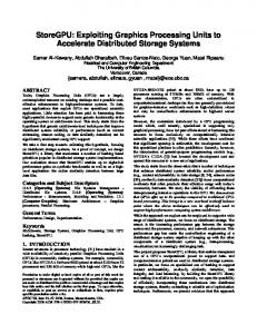
Figure 1: From splines to image warps. (a) A weighted sum of uniformly spaced cubic Bspline basis functions used to construct a C2 continuous curve in one dimension. (b) The previous five basis functions are combined with another four to generate a two-dimensional tensor product; two weighted sums of these 2D basis functions are used to model the x and y components of a displacement vector field. (c) The x displacement field in yellow has been used to deform a regular grid, overlaid in blue. (d) The same transformation illustrated using a brain image: the red edges from the original MRI are overlaid on a grayscale image of the warped result.

17

Reference image

Floating image

Cubic B-Spline interpolation kernel

Control point Positions

Trilinear interpolation kernel

Parzen Window joint histogram filling function

exit

Stopping criteria reached ? yes

Bending-Energy computation kernel

no

Metric value improvement ?

yes

Control point positions update kernels

no

NMI gradient field computation kernel

Bending-Energy gradient computation kernel

NMI gradient field smoothing along X axis NMI gradient field smoothing along Y axis NMI gradient field smoothing along Z axis

Figure 2: Organization of our implementation

18

(a)

(b)

(c)

(d)

(e)

(f)

Figure 3: 3D image registration. By optimising a measure of the similarity of two images (NMI) as a function of the spline weights, a floating image (a) can be automatically brought into alignment (b) with a reference image (c). The initial misalignment is illustrated by alternating between the two images (d) and as a difference image (e-left). The equivalent results after registration are shown in (f) and (e-right). Optimisation of the 40-by-44-by40-by-3 = 211,200 weights is computationally challenging.

19

(a)

(b)

(c)

Figure 4: Examples of manually segmented masks. Segmentation of the amygdala areas are presented on the axial view (b), the blue area on the sagital view (b) corresponds to the entorhinal cortex and the coronal view (c) shows the superior temporal gyra.

20

Mask area

Affine only

classical FFD

Fast-FFD

left amygdala

0.531 (0.163)

0.759 (0.089)

0.776 (0.066)

left entorhinal cortex

0.203 (0.189)

0.296 (0.164)

0.372(0.155)

left fusiform gyrus

0.398 (0.103)

0.483 (0.096)

0.499(0.098)

left hippocampus

0.429 (0.157)

0.658 (0.093)

0.686(0.075)

left medial-inferior temporal gyrus

0.626 (0.070)

0.699 (0.061)

0.709(0.064)

left parahippocampal gyru

0.399 (0.146)

0.527 (0.094)

0.637(0.070)

left superior temporal gyrus

0.607 (0.069)

0.742 (0.057)

0.737(0.048)

left temporal lobe

0.748 (0.052)

0.832 (0.046)

0.827(0.041)

right amygdala

0.571 (0.139)

0.779 (0.072)

0.787 (0.058)

right entorhinal cortex

0.170 (0.177)

0.266 (0.169)

0.334 (0.162)

right fusiform gyrus

0.450 (0.111)

0.542 (0.119)

0.534 (0.113)

right hippocampus

0.479 (0.162)

0.631 (0.120)

0.710 (0.086)

right medial-inferior temporal gyrus

0.662 (0.062)

0.763 (0.059)

0.760 (0.053)

right parahippocampal gyru

0.276 (0.208)

0.323 (0.189)

0.340 (0.275)

right superior temporal gyrus

0.624 (0.055)

0.780 (0.048)

0.775 (0.040)

right temporal lobe

0.733 (0.119)

0.811 (0.128)

0.813 (0.125)

Table 2: Average (standard deviation) results of the segmentation propagation. For each propagation, the Dice similarity value between the manual and the propagated segmentations has been computed.

21