Fast Implementation of ℓ1 Regularized Learning Algorithms Using Gradient Descent Methods∗ Yunpeng Cai†
Yijun Sun‡
Yubo Cheng†
Abstract With the advent of high-throughput technologies, ℓ1 regularized learning algorithms have attracted much attention recently. Dozens of algorithms have been proposed for fast implementation, using various advanced optimization techniques. In this paper, we demonstrate that ℓ1 regularized learning problems can be easily solved by using gradient-descent techniques. The basic idea is to transform a convex optimization problem with a non-differentiable objective function into an unconstrained non-convex problem, upon which, via gradient descent, reaching a globally optimum solution is guaranteed. We present detailed implementation of the algorithm using ℓ1 regularized logistic regression as a particular application. We conduct large-scale experiments to compare the new approach with other stateof-the-art algorithms on eight medium and large-scale problems. We demonstrate that our algorithm, though simple, performs similarly or even better than other advanced algorithms in terms of computational efficiency and memory usage. Keyword: ℓ1 regularized learning, feature selection, sparse solution, gradient descent 1 Introduction High-throughput technologies now routinely produce datasets with unprecedented number of features representing each data sample. ℓ1 regularized learning, due to its ability to produce sparse solutions, has attracted much attention in the last decade. Examples of applications, where this strategy has been shown to be successful, include LASSO [31], generalized LASSO [27], ℓ1 -SVM [32] and ℓ1 regularized logistic regression [20]. ∗ This work is supported in part by Susan Komen Breast Cancer Foundation under grant No. BCTR0707587. Please address all correspondence, including code requests, to: Dr. Yijun Sun (
[email protected]) † Department of Electrical and Computer Engineering, University of Florida, Gainesville, FL 32610 ‡ Interdisciplinary Center for Biotechnology Research, University of Florida, Gainesville, FL 32610 § Cancer Research Institute, M.D. Anderson Cancer Center, Orlando, FL 32827
862
Jian Li†
Steve Goodison§
Despite its attractive properties, the fast implementation of ℓ1 regularized algorithms for high-dimensional data has long been considered a difficult computational problem since the so-obtained objective function is nondifferentiable. Generic methods for non-differentiable convex problems, such as ellipsoid or sub-gradient methods, are typically very slow. In recent years, dozens of algorithms have been developed to deal with medium and large-scale problems, using various advanced optimization techniques. The most commonly used approach is to transform the original problem into one with a convex and differentiable objective function and constraints, and then solve it using standard convex optimization techniques or specified techniques. Due to a large number of constraints, there are only a few methods capable of handling large-scale problems, which mainly fall into two categories. The first category is projected gradient-descent methods (e.g., [1], [5] and [28]). The basic idea is to apply gradient descent methods to minimize an objective function as if there were not constraints, but the infeasible solutions along the gradient direction onto the border of feasible sets. The implementation of these algorithms is very simple. The main drawback, however, is that the projection of infeasible solutions may lead to inaccurate estimates of descending directions, and consequently can significantly slow down the convergence, as is shown in this paper. The methods in the second category employ penaltybased techniques such as interior-point methods [16] to deal with the constraints. Although the interior-point based method is computationally very efficient, its implementation is quite complicated and demands expertise in optimization theories. Moreover, it is a secondorder method that takes advantage of the sparseness of a Hessian matrix. If the data matrix is not sparse, which is the case in many practical applications such as cancer studies using microarray data, both computational complexity and memory usage increase. Another popular approach converts the general ℓ1 learning problem into a series of least-square regression problems, and then solves the so-obtained LASSO model iteratively [19, 27, 18]. These methods require an external LASSO solver and, as we show in our experiments, the
Copyright © by SIAM. Unauthorized reproduction of this article is prohibited.
performance degrades significantly when the number of relevant features becomes excessively large. Other approaches include path-following methods [22, 25], generalized iterative scaling [13, 23], coordinate descent methods [9, 10] and Gauss-Seidel method [29]. There also exist some approaches that modify objective functions to get an approximate solution to ℓ1 regularized algorithms in order to cope with high-dimensional data (see, for example, [2]). The main contribution of this paper is that we show that ℓ1 regularized learning problems can be easily solved by using gradient-descent techniques. We first transform a convex optimization problem with a nondifferentiable objective function into an unconstrained problem. We then prove that if the initial point is properly selected, the solution obtained via gradient descent, when the gradient vanishes, is a global minimizer. We present detailed implementation of the algorithm, using ℓ1 regularized logistic regression as one particular application. Unlike many existing approaches, the implementation is very easy. Moreover, the proposed algorithm is a generic method that can be readily extended to solve other ℓ1 regularized learning problems with minor modifications. Although this paper mainly focuses on batch learning, the proposed method can be readily modified to perform online learning. We present some numerical experiments to compare the new approach with other state-of-the-art algorithms on eight medium and largescale problems. We demonstrate that our algorithm, though simple, performs better than other state-of-theart algorithms in terms of computational efficiency and memory usage. For example, in one of our simulation studies, it takes only 82 seconds for our algorithm to solve a problem with more than two million features, while all other methods fail due to memory limitations. The rest of the paper is organized as follows. Section 2 describes the main idea of the proposed method. Section 3 presents the detailed implementation of the method. Section 4 presents some numerical experiments to compare the new approach with existing algorithms. Section 5 describes briefly how the proposed method can be used to solve ℓ1 -SVM where the loss function is non-differentiable and extended for online learning. The paper is concluded in Section 6 with some concluding remarks. 2
Gradient Descent Based Method for Solving ℓ1 Regularized Problems This section describes the main idea of the proposed method. Let D = {x(n) , yn }N n=1 denote a training dataset, where x(n) ∈ RJ is the n-th pattern and yn ∈ R is the corresponding target value. We seek an optimal solution (w∗ , b∗ ) to the following ℓ1 regularized learning
863
problem: (2.1) N 1 ∑ L(yn , wT x(n) + b) + λ∥w∥1 , w,b N n=1 ∑ where ∥w∥1 = j |wj |, wj is the j-th element of w, L(·) is a loss function, and λ is a regularization parameter that controls the sparseness of the solution. We herein require that L(·) be a convex and twice continuously differentiable function with respect to the second argument. The above formulation encompasses a wide range of learning algorithms, including LASSO [31] and ℓ1 regularized logistic regression algorithm [20]. If a modified hinge loss is used (see, for example, [24, 4]), (2.1) represents an approximate formulation of ℓ1 -SVM. The above formulation has a very appealing property for high-dimensional data analysis. It has been proved in [26] that solving problem (2.1) leads to a globally optimal solution w∗ with at most N non-zero elements. When N ≪ J, it provides an explicit mechanism to perform feature selection to significantly reduce model complexity. This property, however, comes at a price. Unlike ℓ2 regularization, ∥w∥1 is a nondifferentiable function of w. The efficient implementation of ℓ1 regularized formulations poses a computational challenge to the machine learning community. We below demonstrate how a simple gradient descent technique can be used to efficiently solve ℓ1 regularized learning problems. ¯ (n) = [(x(n) )T , −(x(n) )T ]T . Let us conDenote x sider the following optimization problem: (2.2) N 2J ∑ 1 ∑ ¯ (n) + b) + λ min f2 (w, ¯ b) = L(yn , w ¯Tx w ¯i , w,b ¯ N n=1 i=1 ¯ ≥ 0. s.t. w
min
f1 (w, b) =
The following lemma shows that the solution to (2.1) can be recovered from the solution to (2.2). Lemma 2.1. Let (w ¯ ∗ , b∗ ) be an optimal solution to (2.2) where w ¯ ∗ = [(w ¯ ∗(1) )T , (w ¯ ∗(2) )T ]T and ∗(1) ∗(2) J ∗(1) ∗(2) ∗ w ¯ ,w ¯ ∈ R . Then, (w ¯ −w ¯ , b ) is an optimal solution to (2.1). Also, if (w∗ , b∗ ) is an optimal solution to (2.1), then there exist w ¯ o(1) and w ¯ o(2) , so ∗ o(1) o(2) o(1) T o(2) T T ∗ that w = w ¯ −w ¯ and ([(w ¯ ) , (w ¯ ) ] ,b ) is an optimal solution to (2.2). The following lemma shows that at least half of the elements of the optimal solution to (2.2) are zero. We will exploit this property in our algorithm implementation. Lemma 2.2. Let (w ¯ ∗ , b∗ ) be an optimal solution to ∗ (2.2) and w ¯ = [(w ¯ ∗(1) )T , (w ¯ ∗(2) )T ]T , then ∀j ∈ [J] = ∗(1) ∗(2) [1, · · · , J], either w ¯j or w ¯j or both are equal to zero.
Copyright © by SIAM. Unauthorized reproduction of this article is prohibited.
The proof of Lemmas (2.1) and (2.2) is straightforward and hence omitted. The conversion from (2.1) to (2.2) is a standard step that has been previously used in many algorithms (e.g., [28, 5]). Note that (2.2) is a constrained convex optimization problem with a differentiable objective function. In order to use gradient descent, traditional methods usually apply projection or barrier functions to prevent the solution from falling outside the feasible region. In this paper we adopt an essentially different approach, which converts the problem into an unconstrained one. Let w ¯j = vj2 , ∀j ∈ [2J]. Then, (2.2) can be rewritten as (2.3) N 2J 2J ) ∑ 1 ∑ ( ∑ 2 (n) min f (v, b) = L yn , vj x ¯j + b + λ vj2 . N n=1 (v,b) j=1 j=1 After the above transformation, the objective function of (2.3) is no longer convex, which is usually an undesirable property in optimization, except for some rare cases [6, 7]. In the rest of this section, we show that the transformation is beneficial in the sense that it not only preserves the global convergence property of the original problem, but also enables removal of irrelevant variables. Taking the derivatives of f with respect to v and b, respectively, yields (2.4) ( ) ∑2J 2 (n) N ¯j + b) (n) 1 ∑ ∂L(yn , j=1 vj x ∂f ¯ + λ ⊙ v, x ∂v = 2 N n=1 ∂t ∑2J 2 (n) N ¯j + b) 1 ∑ ∂L(yn , j=1 vj x ∂f , ∂b = N ∂t n=1 where ∂L(·)/∂t is the derivative of L with respect to the second argument, and ⊙ is Hadamard operator. For convenience, we denote v ¯ = [vT , b]T and g = ∂f T ∂f T (k) [( ∂v ) , ( ∂b ) ]|. Let v ¯ be the estimates of v ¯ in the k-th iteration and g(k) be the value of g at v ¯(k) . A gradient descent method uses the following updating rule: (2.5)
v ¯(k+1) = v ¯(k) − ηg(k) ,
where η is determined via a line search. Since the objective function of (2.3) is not a convex function, a gradient descent method may find a local minimizer or a saddle point. The following theorems show that if the initial point is properly selected, the solution obtained when the gradient vanishes is a global minimizer.
864
Theorem 2.1. Let f (w, b) be a differentiable convex function of w and b, where w ∈ RJ , w ≥ 0, and b ∈ R. Let g(¯ v) = f (w, b) where w = [w1 , · · · , wJ ]T = ∂g 2 2 T [v1 , · · · , vJ ] and b = vJ+1 . If ∂¯ ¯=¯ v+ = 0, then v |v + v ¯ is not a local minimizer, but a saddle point or a global minimizer of g(¯ v). If the Hessian matrix H(¯ v+ ) + is positive semi-definite, then v ¯ is a global minimizer. Theorem 2.2. For g(¯ v) and v ¯+ defined above, if v ¯+ is found through gradient descent with a line search satisfying the following conditions: 1. interval condition: a line search splits the section under search into a finite number of intervals, 2. descending condition (see the definition below), 3. greedy condition (see the definition below); (0)
and an initial point v ¯(0) satisfying vj ̸=0, ∀j∈[J], then with probability one, v ¯+ is a global minimizer of g(¯ v). Here we give the definitions of the descending and greedy conditions for a line search: Definition 2.1. (descending condition) Let g(¯ v) be an objective function, g(¯ v) be its gradient, v ¯(k) be the solution obtained in the k-th iteration, and −d(k) be the descending direction, a line search is said to satisfy the descending condition if the chosen step length η satisfies d(k)T g(¯ v(k) − ηd(k) ) > 0 . Definition 2.2. (greedy condition) Given g(¯ v) and g(¯ v) defined above, and ϵ(k) be the length of the intervals at the k-th iteration, a line search is said to satisfy the greedy condition if the step length η chosen satisfies g(¯ v(k) − ηd(k) ) ≤ g(¯ v(k) − (η + ϵ(k) )d(k) ), or v ¯(k) − (η + ϵ(k) )d(k) is excluded from the line search; and g(¯ v(k) − ηd(k) ) ≤ g(¯ v(k) − (η − ϵ(k) )d(k) ), or v ¯(k) − (η − ϵ(k) )d(k) is excluded from the line search. The interval condition prevents the algorithms from over-exploring along a gradient descent direction. The descending and greedy conditions ensure that a line search approaches a local optimum along the descending direction, but never hits or goes beyond it. With these conditions a gradient descent method can improve its quality step by step and to be immune from misleading gradient information. Golden section search [15] is an example that satisfies the greedy condition and splits the section into finite intervals according to the golden section rule. We first present the proof of Theorem (2.1).
Copyright © by SIAM. Unauthorized reproduction of this article is prohibited.
∂g ∂g Proof. For simplicity, we use ∂¯ ¯=¯ v∗ . It is easy v∗ to denote ∂¯ v |v Also, we use A ≻ 0 and A ≽ 0 to denote that matrix A is positive definite or semi-definite, respectively. We examine the properties of the Hessian matrix of C= + g(¯ v), denoted as H. Let v ¯ be a stationary point of g(¯ v) satisfying:
(2.6)
[ ]T ∂g ∂f ∂f + + ∂f 2v , · · · , = 2v , =0, ∂¯ v+ ∂w1+ 1 ∂wJ+ J ∂b+
to prove that 2 4vM +1 .. .
...
4vM +1 vJ .. .
4vM +1 vJ 2vM +1
... ...
4vJ2 2vJ
2vM +1 .. . ≽0. 2vJ 1
Hence, by Schur product theorem [14], A2 = (B ⊙ C) v¯=¯v+ is a positive semi-definite matrix. It follows that H(¯ v+ ) ≽ 0 if and only if A1 ≽ 0. If H(¯ v+ ) is not positive semi-definite, then v ¯+ is a saddle point (Note that it cannot be a maximizer because g(¯ v) is convex with respect to vJ+1 and H(¯ v+ ) + + cannot be negative semi-definite). If H(¯ v ) ≽ 0, v ¯ can be either a saddle point, or a local or global minimizer. We now prove that if H(¯ v+ ) ≽ 0, v ¯+ must be a global minimizer. Let us first consider the following optimization problem:
where w+ = [w1+ , · · · , wJ+ ]T = [(v1+ )2 , · · · , (vJ+ )2 ]T and + b+ = vJ+1 . Note that some elements of v ¯+ may be equal to zero. For simplicity and without loss of generality, assume that the first M elements of v ¯+ belong to + + S0 = {vj : vj = 0, 1 ≤ j≤ J}, while the rest J − M elements belong to S̸=0 = {vj+ : vj+ ̸= 0, 1≤j≤J}. From Eq. (2.6), we have ∂f /∂wj+ = 0 for vj+ ∈ S̸=0 . Then, the Hessian matrix of g(¯ v), evaluated at v ¯+ , is given by ( ) (2.9) min f (w, b), subject to w ≥ 0. A1 0 (2.7) H(¯ v+ ) = , 0 A2 Since both the objective function and constraints are convex, the KKT conditions are the sufficient conditions where of a global optimal solution. It can be shown that (2.8) ∂f (w+ , b+ ) is a global minimizer of f (w, b), if for all j ∈ [J] 2 ∂w+ . . . 0 the following KKT conditions hold simultaneously: 1 .. .. , A1 = . . 1. ∂f /∂b+ = 0, ∂f 0 . . . 2 ∂w + M 2. ∂f /∂wj+ = 0, or wj+ = 0 and ∂f /∂wj+ ≥ 0. A3 z Since v ¯+ is a stationary point, by Eq. (2.6), A2 = T ∂2f , z ∀i ∈ {i : vi+ ∈ S̸=0 }, ∂f /∂wi+ = 0 and ∂f /∂b|b=v+ = 0. ∂ 2 b+ J+1 ∂2f ∂2f +2 + + Moreover, H(¯ v+ ) ≽ 0 implies that A1 ≽ 0. Since A1 is . . . 4vM 4vM + +1 ∂ 2 w+ +1 vJ ∂w+ M +1 M +1 ∂wJ a diagonal matrix, it holds that .. .. A3 = , . . 2 2 ∂f /∂wi+ ≥ 0, ∀i ∈ {i : vi+ ∈ S=0 }. ∂ f + + +2 ∂ f 4vM 4v +... + 2 +1 vJ ∂w+ J ∂ wJ M +1 ∂wJ + Hence, by the KKT conditions, (w+ , vJ+1 ) and v ¯+ are [ ]T a global minimizer of f (w, b) and g(¯ v), respectively. ∂2f + + ∂2f z = 2vM . . . 2v . + + + +1 ∂w J ∂w ∂b+ M +1 ∂b J Next, we prove that if the stationary point v ¯+ is found via gradient descent with an initial point v ¯(0) Here we have used the fact that ∂f /∂wj+ = 0 for (0) + satisfying vj ̸= 0, 1 ≤ j ≤ J, then v is a global vj+ ∈ S̸=0 . Since f (w, b) is a convex function of w and minimizer of g(¯ v) with probability one. b, we have Proof. [Theorem 2.2] Suppose that ∂g/∂¯ v∗ = 0 and ∂2f ∂2f ∂2f ∗ . . . 2 v ¯ is a saddle point. Again, we assume that the first ∂wM +1 ∂wJ ∂wM +1 ∂b ∂wM. +1 . . M elements of v ¯∗ belong to S0 , while the following .. .. .. J − M elements belong to S̸=0 . There exists an element ∂2f ∂2f ∂2f B= ≽0. ∂wM +1 ∂wJ . . . ∂wJ 2 ∂wJ ∂b j ∈ S0 so that ∂f /∂wj∗ < 0 (otherwise H(¯ v∗ ) ≽ 0 ∗ and v ¯ is a global minimizer). Due to the continuity, ∂2f ∂2f ∂2f . . . there exists ξ > 0, such that ∂f /∂wj < 0 for every 2 ∂wM +1 ∂b ∂wJ ∂b ∂b
865
Copyright © by SIAM. Unauthorized reproduction of this article is prohibited.
wj ∈ C = {w : |w − wj∗ | < ξ}. It follows that ∂g/∂vj = ξ2 > 0 such that for all v ¯ ∈ C2 = {¯ v| ||¯ v−v ¯(k)− || < √ T (k)− 2vj (∂f /∂wj ) < 0 for vj = wj , and ∂g/∂vj > 0 for ξ2 }, g(¯ v) g > 0. This mean that a gradient√ vj = − wj . That is, a gradient descent method given based search starting in C2 will go pass v ¯(k)− following (k)− (k+1) (k) (k) ¯ is not a point of by vj ← vj − η(∂g/∂vj ), drives the solution out case (2a) stated above, hence v attraction and after a few iterations, case (1) and case of the neighborhood of a saddle point except when (1) (2b) either change to case (2a), or change to the case (k) (k) the component vj is set to exactly zero, or (2) vj is that the descending direction does not drive any element outside C and a line search hits v ¯∗ exactly. The latter towards zero. This completes the proof that the saddle event cannot happen since gradient g(¯ v∗ ) equals to zero points cannot be reached with the designated gradient at v ¯∗ , and thus the descending condition does not hold descent method. (see Definition 2.1). Instead, a line search will find a solution around v ¯∗ , and in the subsequent steps the The correctness of the proof of Theorem (2.2) is solution will move away from v ¯∗ . On the contrary, if v ¯∗ verified experimentally in Section 4. For the above (k+1) is a global optimal, v ¯ will approach it continuously derivations, we can see that the only price we pay to with improved solution quality. transform a convex optimization problem with a non(0) (k) We go on to prove that if vj ̸= 0, vj will be differentiable objective function into an unconstraint set to exactly zero at a non-stationary point with a one is to double the number of variables. Although zero probability. Let v ¯(k) be the solution obtained in the resulting objective function is non-convex, we prove the k-th iteration, −d(k) be the descending direction, that, via gradient descent, reaching a global minimizer is v ¯(k)− = v ¯(k) − ηd(k) be a point in the line-search path guaranteed. Since our method mainly relies on gradient at which some elements are zeros, and g(k)− be the descent, we hereafter refer it as Direct Gradient Method, gradient at v ¯(k)− . Since v ¯(k)− is not a stationary point, or DGM for short. (k)− ||g || > 0. 1. If d(k)T g(k)− ≤ 0, the line search will not reach 3 Implementation Details We present the detailed implementation of DGM, using v ¯(k)− . ℓ1 regularized logistic regression as one particular application. However, using DGM to solve other ℓ1 regular2. On the other hand, If d(k)T g(k)− > 0, −d(k) is ized learning problems is straightforward (see Section also a descending direction at v ¯(k)− . Without 5). loss of generality, we assume ||d(k) || = 1. Due The loss function of ℓ1 regularized logistic regression to the continuity, there exists a ξ1 > 0 such is given by that for all v ¯ ∈ C = {¯ v| ||¯ v−v ¯(k)− || < ξ1 }, d(k)T g(¯ v) > 0. This means that for any α ∈ (0, 1), (3.10) L(y, a) = log(1 + exp(−ya)), g(¯ v(k)− − αξ1 d(k) ) < g(¯ v(k)− ). where label y ∈ {−1, +1}. The gradients of f in Eq. (a) If the chosen interval length ϵ(k) < ξ1 , the line (2.3) with respect to v and b are given by search has at least one candidate solutions ( ) N ( ) which is correspond with an α > 0 above, 1 ∑ ∂f T (n) (n) (k)− ¯ x ¯ + b) x ¯ yn σ −yn (w ⊙v , hence it goes pass v ¯ and moves away from ∂v = 2 λ − N n=1 it. N ( ) 1 ∑ ∂f ¯Tx ¯ (n) + b) , yn σ −yn (w ∂b = − N (b) On the other hand, if ϵ(k) ≥ ξ1 , the line n=1 search will have only one or two candidate solutions within C. In this case, the line respectively, where σ(·) is the sigmoid function. The search has no prior knowledge about the gradient descent steps in (2.5) is then applied. In each line search [21] to region under search, thus it degenerates to step, we first apply back-tracking (e) (e) obtain an end point v ¯ where f (¯ v ) ≤ f (¯ v(k) ), then randomly selecting one or two α ∈ (−1, 1) golden section line search on the section between and setting v ¯(k+1) = v ¯(k)− − αξ1 d(k) . Given apply (k) v ¯ and v ¯(e) . an arbitrary bounded probability density distribution, the probability that a single 3.1 Hybrid Conjugate Gradient Because a simple point α = 0 is chosen, however, is zero. gradient descent method is known to zig-zag in some function contours, we use the Fletcher-Reeves conjugate Moreover, due to the continuity, there also exists a gradient descent method [8] to enhance the performance
866
Copyright © by SIAM. Unauthorized reproduction of this article is prohibited.
of the algorithm: (3.11) v ¯(k+1) d(1) d(k) β
= v ¯(k) − ηd(k) , = g(1) , = g(k) + βd(k−1) , ⟨g(k) , g(k) ⟩ , = ⟨g(k−1) , g(k−1) ⟩
∀k > 1 ,
where d(k) is the conjugate gradient, and ⟨·⟩ is the inner product. Note that conjugate gradient method does not ensure that the objective function decreases monotonically. Hence, when ⟨g(k) , d(k) ⟩ ≤ 0, one usually replaces d(k) with g(k) as the search direction to ensure that the algorithm always proceeds in a descending direction. In our implementation, we adopt a hybrid gradient descent scheme. Denote f (k) as the objective function obtained in the k-th iteration and ∠(a, b) the angle between vectors a and b. If (f (k) − f (k−1) )/f (k) < θ1 and ∠(g(k) , d(k) ) < θ2 , we use −d(k) as the descending direction, and −g(k) otherwise. In our implementation, we set θ1 = 0.01 and θ2 = 5/12π. It should be noted that with the descending condition, the global convergence property also holds for conjugate gradient descent. In Section 2 we stated that the solution w ¯ ∗ has at most min(N, J) non-zero elements. We exploit this property to speed up the implementation. Note in (2.4) that if vj = 0, then the gradient will be zero on the j-th element, and vj will remain zero thereafter. Hence, if some elements of v are extremely small, the corresponding features can be eliminated from further consideration with a negligible impact on the subsequent iterations and the final solution found. In our implementation, the criterion for eliminating small-valued weights is wj < 10−10 ∥w∥∞ , where ∥w∥∞ = maxj {wj }. From the discussion in the last section, we can see that if the threshold is small enough that it is always far smaller than ξ1 in any step, the purging will be safe. The implementation of DGM is very easy. The pseudo-code is given in Algorithm 1. 3.2 Computational Complexity With conjugate gradient descent, in each iteration, the flops needed to compute gradient is O(N J), and the memory required is O(N + J), where N is the sample size and J the data dimensionality. For comparison, the interior point method for ℓ1 logistic regression requires O(N 2 J) flops if J > N , and O(N J 2 ) if N > J. Hence, the computational complexity of the interior point method is much higher than DGM, though the interior point method, as a second-order method, usually requires fewer iterations.
867
Algorithm 1: DGM Algorithm J Input : Data D = {(x(n) , yn )}N n=1 ⊂ R × {±1}, parameters θ1 , θ2 , a stopping criterion Output: w, b √ (0) 1 Initialization: Set v = 1/ (2J), b(0) = 0, t = 0; ¯ (0) = [(v(0) )T , b]T ; 2 v (0) 3 Compute f using Eq. (2.3); 4 repeat 5 t = t + 1; Compute g(t) using Eq. (3.11); 6 7 if t > 1 and ∥f (t) − f (t−1) ∥/∥f (t) ∥ < θ1 then Compute d(t) using Eq. (3.11); 8 9 if ∠(g(t) , d(t) ) ≥ θ2 then 10 d(t) = g(t) ; 11 end 12 end 13 else 14 d(t) = g(t) ; 15 end ¯ (t) = v ¯ (t−1) − η (t) d(t) , where η (t) is Update v 16 determined via line search; (t) 17 if v¯i < 10−5 ∥¯ v(t) ∥∞ , ∀i ∈ [2J] then (t) 18 v¯i = 0; 19 end 20 until stopping criterion ; (t) (t) ¯ (1) = [(¯ 21 w vJ )2 ]T ; v1 )2 , · · · , (¯ (t)
(t)
23
¯ (2) = [(¯ w vJ+1 )2 , · · · , (¯ v2J )2 ]T ; ¯ (1) − w ¯ (2) ; w=w
24
b = v¯2J+1 .
22
4
(t)
Numerical Experiments
We present some numerical experiments to compare DGM with five state-of-the-art methods, namely, interior point method [16], logistic LARS [18], ProjectL1 [28], the ℓ1 ball projection [5] and Orthant-Wise Limited-memory Quasi-Newton (OWLQN) [1]. These methods cover almost all recently proposed methods on general ℓ1 regularized learning. They have been extensively tested on a wide variety of data sets and compared against dozens of other methods, including GenLASSO [27], iterated scaling [13], BBR [10] and some traditional gradient-based methods. It is reported that these methods are one or two orders of magnitude faster than existing methods. Hence, we believe that the comparison with these methods is sufficient to demonstrate the effectiveness of our newly proposed method.
Copyright © by SIAM. Unauthorized reproduction of this article is prohibited.
4.1 Experiment Setup We apply each algorithm to eight data sets using a specified set of λ values. Each algorithm stops when the achieved objective function is within 10−6 precision of the optimal solution. The CPU time of each algorithm is then recorded and compared. The time spent on loading data and writing solutions is excluded from the CPU time. The interior point method solves (2.1) and its dual problem simultaneously, and computes the duality gap that is used as the upper bound of the precision. The maximum of the dual problem is used as the lower bound of the minimum of the primal problem. In contrast, other methods adopt a different stopping criterion, namely, the difference of the objective functions in two consecutive iterations. To make a fair comparison, in our experiments, for every data set and λ value, we first run the interior point method, which stops when the duality gap is within a desired precision. After that, we set the so-obtained objective function of the dual problem in the interior point method as the target value of the other methods. By using this experimental protocol, we verify that the solution obtained by DGM is indeed a global minimizer. It should be noted that logistic LARS and ℓ1 ball projection solve a different problem: min w,b
N 1 ∑ L(yn , wT x(n) + b) N n=1
s.t. ∥w∥1 ≤ C .
In order to obtain a comparable solution with other algorithms, after running DGM and the interior point method, we compute the 1-norm of the obtained w and use it as the upper bound C in logistic LARS and ℓ1 ball projection. We use the method described in [16] to determine the proper range of λ. The upper bound of a possible λ can be calculated as:
|S − | ∑
+ ∑ |S |
λmax = x(n) − x(n) ,
N
N + − n∈S
n∈S
∞
where S + = {n| yn = 1} and S − = {n| yn = −1}. We set λ to be uniformly spaced on a logarithmic scale over interval [0.001λmax , 0.99λmax ], which covers the range of interest for most practical applications. The interior point method and OWLQN are coded in C. Logistic LARS is programmed in matlab and C-mex mixed code with all computationally intensive tasks executed in C, and thus is almost as efficient as pure C program. ProjectionL1 is coded in Matlab only. Hence, we develop both C and Matlab versions of DGM for comparison. Since ℓ1 ball projection does not have a published code, we implement it in
868
Table 1: Summary of data sets Data No. of features No. of samples Colon cancer 2000 62 Leukemia 7129 72 Internet Ads. 1430 2359 Prostate cancer 22291 79 TABM77 1145 291 GSE4922 44932 249 Arcene 10000 200 Linear 10000 400
Matlab by strictly following the instructions provided by [5]. The batch-learning version of the algorithm is implemented. The algorithm needs to specify an initial step length, or determine it via back-tracking line search. We implement both line-search and nonline-search versions, tune the initial step length of the non-line-search version for all data sets and all λ within a wide range of [108 , 10−8 ], and report the best results, which outperform the line-search one reported in [5]. The first experiment described below is performed on a personal computer with Intel Core 2 T5500 1.66GHz CPU, 512MB memory, and Linux operating system. The second experiment, due to memory requirements, is run on an Intel Xeon 2.83G server with 8GB memory and Window XP operating system, where the system allows a maximum of 2GB memory. 4.2 Experimental Results We first compare the algorithms on eight medium and large-scale data sets with feature dimensionality ranging from 1, 000 to 44, 932. Among them, internet ads, leukemia and colon cancer gene expression data have already been used in [16, 18]. The arcene data is first used in the NIPS feature selection challenge [11], and prostate cancer [30], ETABM77 [3] and GSE4922 [12] are three cancer microarray data. The Linear data is an artificially generated binary classification problem, with each class having 200 samples characterized by 104 features. The first 500 features are drawn from two normal distributions N (−1, 1) and N (1, 1), depending on class labels. The rest of the features are drawn from the standard normal distribution, thus providing no discriminant information. The summary of the data is given in Table 1. In practical applications, cross validation is usually performed over all possible λ values to estimate the optimal regularization parameter λ. We apply the six algorithms to eight data sets, and record in Table 2 the total running time summed over seven λ values uniformly spaced on a logarithmic scale over interval [0.001λmax , 0.99λmax ]. We observe that in seven out of
Copyright © by SIAM. Unauthorized reproduction of this article is prohibited.
Solving Time vs. λ 3
DGM IP logLARS ProjL1 L1Ball OWLQN
10
2
Direct Gradient Interior Point 2
10
O( n1.44) CI=[1.33,1.54]
1
1
10
time/s
time/s
10
Solving Time vs. Problem Size
3
10
0
10
10
0
10
0.922
O( n 0
0.5
1
1.5
2
2.5
3
−log(λ/λmax)
) CI=[0.872,0.972]
−1
10
Figure 1: Running time (in seconds) of the six algorithms performed on the prostate cancer dataset using different λ values.
eight data sets, the C version of DGM performs the best, and in seven out of eight data sets, the Matlab version of DGM outperforms ProjectionL1. For some data sets (e.g., arcene and prostate cancer), DGM is one order of magnitude faster than ProjectionL1. ℓ1 ball projection performs very well on the Linear data set, which is consistent with the result reported in [5]. However, in six out of the seven real-world data sets, it performs poorly and cannot reach the targeted precision level in a short time even if we use 10−4 as a stop criterion. OWLQN is significantly slower than all other methods on all data sets, because it mainly focuses on reducing the memory usage, though our method is also memory efficient. Figure 1 depicts the CPU time of the six algorithms performed on the prostate cancer data set using different λ values. We can see that when λ is large, logistic LARS, Projection L1 and ℓ1 ball projection are very fast because the search area is shrunk to a very small region. However, with the decreasing value of λ, the running time of both Projection L1 and ℓ1 ball projection increases dramatically. In contrast, the computational complexity of both DGM and the interior point method does not change significantly with respect to the regularization parameter. The above observation is consistent over the other seven data sets. To further demonstrate the scaling property of our method, we compare DGM and the interior point method using a series of artificially generated linear data set with 200 samples, varying the feature dimensionality from 500 to 2.15 × 10⁶ . Figure 2 presents the CPU time
869
2
10
3
10
4
10
5
10
Problem Dimension Figure 2: Scalability of DGM and the interior point method performed on data sets with feature dimensionality ranging from 102.66 to 106.33 . The empirical complexity and confidence interval (CI) are also reported.
of DGM and the interior point method as a function of data dimensionality. We observe that the solving time of DGM exhibits a sub-linear growth of O(n0.92 ), while for the interior point method the solving time grows super-linearly (O(n1.44 )) with respect to the sample size, which is consistent with the results reported in [16]. For example, when the data dimension is 106 , it takes the interior point method 1017 seconds to solve the problem, while for our method the solving time is only 38 seconds. Moreover, our DGM method uses less memory than the interior point method. For this reason, DGM solves a 2150000-dimensional problem in only 82 seconds using a 2GB memory, while the interior point method fails. From the above observations, we conclude that DGM, though simple, can achieve competitive computational efficiency compared with the state-of-the-art methods. 5 Extensions of DGM DGM is a generic method that can be used to solve various ℓ1 regularized learning problems provided that the loss function is differentiable. The hinge loss used in SVM, however, is a non-differentiable function. We below give a brief discussion on how our method can be used to solve ℓ1 -SVM. One possible way is to replace the
Copyright © by SIAM. Unauthorized reproduction of this article is prohibited.
Table 2: CPU time (in seconds) of the six algorithms performed on the eight data sets. The algorithms stop when the achieved objective function is within 10−6 precision of the optimal solution. The results marked with * are obtained by using 10−4 as a stop criterion. Data DGM-C Interior Point Logistic LARS OWLQN DGM-Matlab Projection L1 L1 Ball Proj.
Colon 15 33 28 466 131 591 6908∗
Leukemia 49 120 80 3442 176 1723 > 24 hr∗
Internet Ads. 226 15 1163 776 665 491 3547
hinge loss with a differentiable function. [4] suggests to use the Huber loss, given by 0 (1 + h − ya)2 L(y, a) = 4h 1 − ya
ya > 1 + h , 1 − h ≤ ya ≤ 1 + h , ya < 1 − h ,
where h is a tunable parameter. If h is sufficiently small, SVM using the Huber loss provides the same sparse solution as SVM with the hinge loss [4]. Hence, with minor modifications, DGM described in Section 2 can be directly used to solve ℓ1 -SVM in the primal domain. Due to its non-constrained formulation, the proposed method can be readily extended for online learning for applications where both the numbers of features and samples are excessively large [17]. By using the theory of stochastic gradient, the convergence is guaranteed. The experimental results of online DGM is reported elsewhere. 6
Conclusions
In this paper we have proposed a simple yet very efficient method to solve ℓ1 regularized learning problems. We have conducted large-scale numerical experiments to demonstrate that our method can achieve improved computational efficiency over the state-of-the-art methods. The proposed method can deal with various loss functions such as the least square loss, hinge loss and truncated least square loss, and can be adopted in both batch learning and online learning scenarios. This work provides a new direction for fast implementation of large-scale ℓ1 regularized learning algorithms. References
[1] G. Andrew, and J.F. Gao, Scalable Training of L1Regularized Log-Linear Models, Proc. 24th Intl. Conf. Mach. Learn., Corvallis, OR, USA, 2007, pp. 33–40.
870
Prostate 82 384 274 32822 209 6783 > 24 hr∗
ETABM77 63 99 116 641 235 268 24234∗
GSE4922 313 3219 2344 > 24hr 959 > 24 hr > 24 hr∗
Arcene 393 788 > 24 hr 25543 2237 32194 > 24 hr∗
Linear 151 1221 1866 5861 492 1821 291
[2] S. Balakrishnan, and D. Madigan, Algorithms for sparse linear classifiers in the massive data setting, J. Mach. Learn. Res., 9 (2008), pp. 313–337. [3] M. Buyse, S. Loi, L. van’t Veer, G. Viale, M. Delorenzi, A. M. Glas, M. S. d’Assignies, J. Bergh, R. Lidereau, P. Ellis, A. Harris, J. Bogaerts, P. Therasse, A. Floore, M. Amakrane, F. Piette,E. Rutgers, C. Sotiriou, F. Cardoso, and M. J. Piccart, Validation and clinical utility of a 70-gene prognostic signature for women with node-negative breast cancer. J. N. Cancer Inst., 98(17) (2006), pp. 1183–1192. [4] O. Chapelle, Training a support vector machine in the primal, Neural Comput., 19 (2007), pp. 1155–1178. [5] J. Duchi, S. Shalev-Shwartz, Y. Singer, and T. Chandra, Efficient projections onto the L1-ball for learning in high dimensions, Proc. 25th Intl. Conf. Mach. Learn., Helsinki, Finland, 2008, pp. 272–279. [6] Y. G. Evtushenkjo and V. G. Zhadan, Spacetransformation technique: the state of the art, in Nonlinear Optimization and Applications, (1996), pp 101– 123. [7] L. Faybusovich, Dynamical systems which solve optimization problems with linear constraints, IMA J. Math. Ctrl. and Info., 8 (1991), pp 135–149; [8] R. Fletcher, Practical methods of optimization, John Wiley, New York, 1997. [9] J. Friedman, T. Hastie, H. Hoefling and R. Tibshirani, Pathwise coordinate optimization, Ann. Appl. Stat., 1 (2007), pp. 302–332. [10] A. Genkin, D. Lewis, and D. Madigan, Largescale bayesian logistic regression for text categorization, Technometrics, 49 (2007), pp. 291–304. [11] I. Guyon, S. R. Gunn, A. Ben-Hur and G. Dror, Result analysis of the NIPS 2003 feature selection challenge, 17th Adv. Neu. Info. Proc. Sys., Vancouver, Canada, (2005), pp. 545–552. [12] A. V. Ivshina, J. George, O. Senko, B. Mow, T. C. Putti, J. Smeds, T. Lindahl, Y. Pawitan, P. Hall, H. Nordgren, J. E. Wong, E. T. Liu, J. Bergh, V. A. Kuznetsov, and L. D. Miller, Genetic reclassification of histologic grade delineates new clinical subtypes of breast cancer, Cancer Res., 66(21) (2006), pp. 10292– 10301.
Copyright © by SIAM. Unauthorized reproduction of this article is prohibited.
[13] J. Goodman, Exponential priors for maximum entropy models, Proc. 42nd Ann. Meet. Asso. Comp. Ling., Barcelona, Spain, 2004, pp. 305–312. [14] R. Horn, and C. Johnson, Matrix analysis. Cambridge University Press, Cambridge, 1985. [15] J. Kiefer, Sequential minimax search for a maximum, Proc. 4th Amer Math. Soc., (1953), pp. 502–506. [16] K. Koh, S. J. Kim, and S. Boyd, An interior-point method for large-scale ℓ1 -regularized logistic regression, J. Mach. Learn. Res., 8 (2007), pp. 1519–1555. [17] J., Langford, L., Li, and T., Zhang, Sparse Online Learning via Truncated Gradient, J. Mach. Learn. Res., 10 (2009), pp. 777–801. [18] S. I., Lee, H., Lee, P., Abbeel, and A. Y., Ng, Efficient ℓ1 regularized logistic regression, Proc. 21st AAAI Conf. Artif. Intell., Boston, MA, USA, 2006, pp. 1–9. [19] J. Lokhorst, The lasso and generalised linear models, Tech. Report, Dept. of Stat., Univ. of Adelaide, Australia, 1999. [20] A. Y. Ng, Feature selection, L1 vs. L2 regularization, and rotational invariance, Proc. 21st Intl. Conf. Mach. Learn., Banff, Alberta, Canada, 2004, pp. 78–86. [21] J. Nocedal, and S. J. Wright, Numerical optimization, Springer Verlag, New York, NY, 1999. [22] M. Park, and T. Hastie, L1 regularization-path algorithm for generalized linear models, J. R. Stat. Soc. Ser. B Stat. Meth., 69 (2007), pp. 659–677. [23] S. Perkins, and J. Theiler, Online feature selection using grafting, Proc. 20th Intl. Conf. Mach. Learn., Washington, DC , USA, 2003, pp. 592–599. [24] J. D. Rennie, and N. Srebro, Fast maximum margin matrix factorization for collaborative prediction, Proc. 22nd Intl. Conf. Mach. Learn., Bonn, Germany, 2005, pp. 713–719. [25] S. Rosset, Following curved regularized optimization solution paths, Proc. 17th Adv. Neu. Info. Proc. Sys., Whistler, Canada, 2005, pp. 1153–1160. [26] S. Rosset, J. Zhu, and T. Hastie, Boosting as a regularized path to a maximum margin classifier, J. Mach. Learn. Res., 5 (2004), pp. 941–973. [27] V. Roth, The generalized LASSO, IEEE Trans. Neu. Net., 15 (2004), pp. 16–28. [28] M. Schmidt, G. Fung, and R. Rosales, Fast optimization methods for L1 regularization: a comparative study and two new approaches, Proc. 18th Euro. Conf. Mach. Learn., Warsaw, Poland, 2007, pp. 286–297. [29] S. Shevade, and S. Keerthi, A simple and efficient algorithm for gene selection using sparse logistic regression, Bioinformatics, 19 (2003), pp. 2246–2253. [30] A. J. Stephenson, A. Smith, M. W. Kattan, J. Satagopan, V. E. Reuter, P. T. Scardino and W. L. Gerald, Integration of gene expression profiling and clinical variables to predict prostate carcinoma recurrence after radical prostatectomy, Cancer, 104 (2005), pp. 290–298. [31] R. Tibshirani, Regression shrinkage and selection via the LASSO, J. R. Stat. Soc. Ser. B, 58 (1996), pp. 267– 288. [32] J. Zhu, S. Rosset, T. Hastie, and R. Tibshirani, 1-
871
norm support vector machines, Proc. 16th Adv. Neu. Info. Proc. Sys., Whistler, Canada, 2002, pp. 49–56.
Copyright © by SIAM. Unauthorized reproduction of this article is prohibited.