Efficient L1 Regularized Logistic Regression

Efficient L1 Regularized Logistic Regression Su-In Lee, Honglak Lee, Pieter Abbeel and Andrew Y. Ng Computer Science Department Stanford University Stanford, CA 94305

Abstract L1 regularized logistic regression is now a workhorse of machine learning: it is widely used for many classification problems, particularly ones with many features. L1 regularized logistic regression requires solving a convex optimization problem. However, standard algorithms for solving convex optimization problems do not scale well enough to handle the large datasets encountered in many practical settings. In this paper, we propose an efficient algorithm for L1 regularized logistic regression. Our algorithm iteratively approximates the objective function by a quadratic approximation at the current point, while maintaining the L1 constraint. In each iteration, it uses the efficient LARS (Least Angle Regression) algorithm to solve the resulting L1 constrained quadratic optimization problem. Our theoretical results show that our algorithm is guaranteed to converge to the global optimum. Our experiments show that our algorithm significantly outperforms standard algorithms for solving convex optimization problems. Moreover, our algorithm outperforms four previously published algorithms that were specifically designed to solve the L1 regularized logistic regression problem.

Introduction Logistic regression is widely used in machine learning for classification problems. It is well-known that regularization is required to avoid over-fitting, especially when there is a only small number of training examples, or when there are a large number of parameters to be learned. In particular, L1 regularized logistic regression is often used for feature selection, and has been shown to have good generalization performance in the presence of many irrelevant features. (Ng 2004; Goodman 2004) Unregularized logistic regression is an unconstrained convex optimization problem with a continuously differentiable objective function. As a consequence, it can be solved fairly efficiently with standard convex optimization methods, such as Newton’s method or conjugate gradient. However, adding the L1 regularization makes the optimization problem computationally more expensive to solve. If the L1 regularization is enforced by an L1 norm constraint on the paramec 2006, American Association for Artificial IntelliCopyright ° gence (www.aaai.org). All rights reserved.

ter vector, then the optimization problem becomes a constraint optimization problem with the number of constraints equal to twice the number of parameters to be learned. The running time of standard algorithms to solve convex optimization problems increases with the number of constraints. If, alternatively, the L1 regularization is implemented by adding (a constant times) the L1 norm of the parameter vector to the objective, then the objective is not continuously differentiable anymore. This precludes the use of, for example, Newton’s method to solve the optimization problem efficiently. Thus, both formulations of L1 regularized logistic regression lead to a more complicated optimization problem than unregularized logistic regression. However, the L1 constraint (or penalty term) has significant structure. For example, if one knew a priori the signs of each of the parameters, then the L1 constraint would become a single linear constraint. Or, in case of regularization by adding the L1 term to the objective, the L1 term would become linear, resulting in a continuously differentiable objective. These (and similar) observations have led to various algorithms that try to exploit the structure in the optimization problem and solve it more efficiently. Goodman (2004) proposed an algorithm for learning conditional maximum entropy models (of which logistic regression is a special case) with an exponential prior (also referred to as a one-sided Laplacian prior). His algorithm is based on generalized iterative scaling (GIS). The idea is to iteratively (efficiently) maximize a differentiable lower bound of the objective function. The proposed learning algorithm can easily be extended to the case of logistic regression with a Laplacian prior by duplicating all the features with the opposite sign. Logistic regression with a Laplacian prior is equivalent to L1 regularized logistic regression. Perkins et al. (2003) proposed a method called grafting. The key idea in grafting is to incrementally build a subset of the parameters, which are allowed to differ from zero. Grafting uses a local derivative test in each iteration of the conjugate gradient method, to choose an additional feature that is allowed to differ from zero. This way, the conjugate gradient method can be applied without explicitly dealing with the discontinuous first derivatives. Roth (2004) proposed an algorithm called generalized LASSO that extends a LASSO algorithm proposed by Osborne et al. (2000). (The LASSO refers to an L1 regularized

least squares problem. See, Tibshirani (1996) for details.) In this paper, we propose a new, efficient algorithm for solving L1 regularized logistic regression. Our algorithm is based on the iteratively reweighted least squares (IRLS) formulation of logistic regression. More specifically, in each iteration, our algorithm finds a step direction by optimizing the quadratic approximation of the objective function at the current point subject to the L1 norm constraint. The IRLS formulation of logistic regression allows us to (iteratively) reformulate the quadratic approximation as a least squares objective. Thus our algorithm ends up solving an L1 constrained least squares problem in every iteration. The L1 constrained least squares problem can be solved very efficiently using least angle regression (LARS), proposed by Efron et al. (2004). Our theoretical results show that our algorithm is guaranteed to converge to a global optimum. (In fact, our theoretical results could be generalized to a larger family of optimization problems, as discussed later.) Our experiments show that our algorithm significantly outperforms the previously proposed algorithms for L1 regularized logistic regression. Our algorithm also significantly outperforms standard gradient-based algorithms, such as conjugate gradient and Newton’s method.1 We note that Lokhorst (1999) also proposed an algorithm that uses the IRLS formulation of logistic regression. However he used a different LASSO algorithm (Osborne, Presnell, & Turlach 2000) in the inner loop and did not provide any formal convergence guarantees.

L1 Regularized Logistic Regression We consider a supervised learning task where we are given M training instances {(x(i) , y (i) ), i = 1, . . . , M }. Here, each x(i) ∈ RN is an N -dimensional feature vector, and y (i) ∈ {0, 1} is a class label. Logistic regression models the probability distribution of the class label y given a feature vector x as follows: 1 p(y = 1|x; θ) = σ(θ> x) = . 1 + exp(−θ> x)

θ

M X

− log p(y (i) |x(i) ; θ) + βkθk1 .

(1)

(2)

i=1

This optimization problem is referred to as L1 regularized logistic regression. Often, it will be convenient to consider 1

min θ

The standard gradient-based algorithms are not directly applicable, because the objective function of the L1 regularized logistic regression has discontinuous first derivatives. In our experiments, we used a smooth approximation of the L1 loss function.

M X

− log p(y (i) |x(i) ; θ),

(3)

i=1

subject to kθk1 ≤ C. The optimization problems (2) and (3) are equivalent, in the following sense: for any choice of β, there is a choice of C such that both optimization problems have the same minimizing argument. This follows from the fact that, (up to a constant that does not depend on θ) the optimization problem (2) is the Lagrangian of the constrained optimization problem (3), where β is the Lagrange multiplier. (Rockafellar 1970) In practice, C (and/or β) may be either chosen manually or via cross-validation; for the sake of simplicity, in this paper, we will consider solving the problem (3) for a given, fixed, value of C.

Our Learning Algorithm In this section, we describe our learning algorithm for L1 regularized logistic regression. We also formally prove that our learning algorithm converges to the global optimum of the optimization problem (3).

Preliminaries IRLS for unregularized logistic regression Our learning algorithm is based on iteratively reweighted least squares (IRLS). (Green 1984; Minka 2003) IRLS reformulates the problem of finding the step direction for Newton’s method as a weighted ordinary least squares problem. Consider the problem of finding the maximum likelihood estimate (MLE) of the parameters θ for the unregularized logistic regression model. The optimization problem can be written as: min θ

Here θ ∈ RN are the parameters of the logistic regression model; and σ(·) is the sigmoid function, defined by the second equality. Under the Laplacian prior p(θ) = (β/2)N exp(−βkθk1 ) (with β > 0), the maximum a posteriori (MAP) estimate of the parameters θ is given by: min

the following alternative parameterization of the L1 regularized logistic regression problem:

M X

− log p(y (i) |x(i) ; θ).

(4)

i=1

In every iteration, Newton’s method first finds a step direction by approximating the objective by the second order Taylor expansion at the current point, and optimizing the quadratic approximation in closed-form. More specifically, let θ(k) denote the current point in the k’th iteration. Then Newton’s method finds a step direction by computing the optimum γ (k) of the quadratic approximation at θ(k) as follows: (k) γ (k) = θ(k) − H−1 (θ(k) )g(θ ). (5) Here H(θ) and g(θ) represent the Hessian and gradient of the objective function in (4) evaluated at θ. Once the step direction γ (k) is computed, Newton’s method computes the next iterate θ(k+1) = (1 − t)θ(k) + tγ (k)

(6)

by a line search over the step size parameter t. We now show how the Newton step direction can be computed by solving a weighted ordinary least squares problem

rather than using Equation (5). (See Green 1984, or Minka 2003 for details of this derivation.) Let X(∈ RN ×M ) denote the design matrix: X = [x(1) x(2) . . . x(M ) ]. Let the diagonal matrix Λ and the vector z be defined as follows: for all i = 1, 2, . . . , M : Λii

=

σ(θ(k)> x(i) )[1 − σ(θ(k)> x(i) )],

zi

=

x(i)> θ(k) +

(7)

[1 − σ(y (i) θ(k)> x(i) )]y (i) . (8) Λii

Then, we have that H(θ(k) ) = −XΛX> and g(θ(k) ) = XΛ(z − X> θ(k) ), and thus Equation (5) can be rewritten as: γ (k) = (XΛX> )−1 XΛz.

(9)

(k)

Thus γ is the solution to the following weighted least squares problem: 1 2

1 2

γ (k) = arg min k(Λ X> )γ − Λ zk22 . γ

IRLS for L1 regularized logistic regression For the case of L1 regularized logistic regression, as formulated in Equation (3), the objective is equal to the unregularized logistic regression objective. By augmenting the IRLS formulation of the unregularized logistic regression with the L1 constraint, we get our IRLS formulation for L1 regularized logistic regression (leaving out the dependencies on k for clarity): 1

1

γ

Our algorithm Our algorithm iteratively solves the L1 constrained logistic regression problem of Equation (3). In the k’th iteration, it finds a step direction γ (k) by solving the constrained least squares problem of Equation (11). Then it performs a backtracking line search (see Boyd & Vandenberghe, 2004 for details) over the step size parameter t ∈ [0, 1] to find the next iterate θ(k+1) = (1 − t)θ(k) + tγ (k) . To summarize, we propose the following algorithm, which we refer to as IRLSLARS. (We discuss the stopping criterion used in more detail when discussing our experimental setup and results.) Algorithm 1 IRLS-LARS

(10)

Therefore, the Newton step direction can be computed by solving the least squares problem (10), and thus the logistic regression optimization problem can be solved using iteratively reweighted least squares (IRLS). This least squares formulation will play an important role in our algorithm. The term IRLS refers to the fact that in every iteration the least squares problem of Equation (10) has a different diagonal weighting matrix Λ and “right-hand side” z, but the same design matrix X. (Note that, although we did not make the dependence explicit, the diagonal matrix Λ and the vector z both depend on θ(k) and therefore change in every iteration.)

min k(Λ 2 X> )γ − Λ 2 zk22 ,

squares problems. In our algorithm, we use LARS with the LASSO modification. (Efron et al. 2004) LARS with the LASSO modification uses a stagewise procedure, based on a simple incremental update, to efficiently solve the L1 regularized least squares problem.

(11)

subject to kγk1 ≤ C Our algorithm (presented in more detail below) iteratively solves the L1 regularized logistic regression problem by (in every iteration) first solving the L1 constrained least squares problem (11) to find a step direction and then doing a line search to determine the step size. Thus our algorithm combines a local quadratic approximation with the global constraints. LARS for solving L1 constrained least squares. The L1 constrained least squares problem of Equation (11) is also known as a LASSO problem. (Tibshirani 1996) Several algorithms have been developed to solve L1 constrained least

1 2 3 4 5 6 7 8 9 10

Set θ(0) = ~0. for (k = 0 to MaxIterations) Compute Λ and z using Equation (7) and Equation (8) (for θ = θ(k) ). Use LARS to solve the L1 constrained least squares problem of Equation (11), and let γ (k) be the solution. Set θ(k+1) = (1 − t)θ(k) + tγ (k) , where t is found using a backtracking line-search that minimizes the objective function given in Equation (3). Evaluate the objective function, given in Equation (3) at θ(k+1) . if (the stopping criterion is satisfied) Break; end end

We note that our algorithm can be applied to, not only L1 constrained logistic regression, but rather to any L1 constrained optimization problems, so long as the unconstrained problem can be solved using IRLS. In particular, our algorithm can be used for parameter learning for L1 constrained generalized linear models. (Nelder & Wedderbum 1972; McCullagh & Nelder 1989)

Convergence and optimality guarantees The following theorem shows that the IRLS-LARS algorithm presented in this paper converges to a global optimum.2 Theorem 1. The IRLS-LARS algorithm presented in the paper converges to a global optimum of the L1 constrained regularized logistic regression problem of Equation (3). 2 In fact—although the theorem statement is specific to our algorithm—the proof easily generalizes to any algorithm that iteratively minimizes the local quadratic approximation subject to the constraints (followed by a line search) so long as the objective function has a continuous 3rd order derivative, and the feasible set is convex, closed and bounded.

Proof. Our convergence proof uses the following fact: Fact 1. Let any point θ0 that is not a global optimum be given. Then there is an open subset Sθ0 that includes θ0 , and there is a constant Kθ0 > 0 such that the following holds: for all feasible φ0 ∈ Sθ0 we have that one iteration of our algorithm, starting from φ0 , will give us a (feasible) point φ1 that satisfies f (φ1 ) ≤ f (φ0 ) − Kθ0 . Proof of Fact 1. We have a convex objective function f with convex constraints. Since θ0 is not a global optimum, any open set that includes θ0 includes a feasible point with strictly lower value of the objective function f . (In fact, all points on a line segment connecting θ0 with a global optimum are feasible and have a strictly lower value of the objective function f .) The objective f is convex and has bounded second derivative over the feasible set, thus for any sufficiently small open set that includes θ0 , we have that this set includes a feasible point with strictly lower value of the local quadratic approximation at θ0 , which we denote by f˜θ0 . Thus when our algorithm globally optimizes the quadratic approximation over the feasible set, the resulting point θ1 must satisfy f˜θ0 (θ1 ) < f˜θ0 (θ0 ). Now define δ > 0 as follows: δ = f˜θ (θ0 ) − f˜θ (θ1 ). (12) 0

0

Since f is three times continuously differentiable and since the feasible set is bounded, there exists ² > 0, such that for all φ0 ∈ Sθ0 = {θ : kθ − θ0 k2 ≤ ²} the following hold: δ |f (θ0 ) − f (φ0 )| ≤ , (13) 8 and for all θ in the feasible set: δ |f˜θ0 (θ) − f˜φ0 (θ)| ≤ . (14) 8 From Equation (14) we have for all φ0 ∈ Sθ0 that | minθ f˜θ0 (θ) − minθ f˜φ0 (θ)| ≤ 4δ .

(15)

Therefore, for all φ0 ∈ Sθ0 the following holds. Let φ1 be the global optimum (within the feasible set) of the quadratic approximation at φ0 , then we have that: f˜φ0 (φ1 )

δ ≤ f˜θ0 (θ0 ) − δ + 4 3δ = f (θ0 ) − 4

0

0

δ ≤ f (φ0 ) − t . (17) 2 Here we used, in order: f˜φ0 is convex; f˜φ0 (φ0 ) = f (φ0 ) and Equation (16). Since f is three times continuously differentiable and the feasible set is bounded, there exists C > 0, such that for all φ0 ∈ Sθ0 the following holds for all θ in the feasible set: f (θ) ≤ f˜φ0 (θ) + Ckθ − φ0 k32 .

(18)

Now, we choose θ = φ0 + t(φ1 − φ0 ) in Equation (18), and we use Equation (17) to obtain: f (φ0 + t(φ1 − φ0 )) ≤ f (φ0 ) − t 2δ + Ckt(φ1 − φ0 )k32 . (19) Let R be the radius of a sphere that includes the (bounded) feasible set, then we get that f (φ0 + t(φ1 − φ0 )) ≤ f (φ0 ) − t 2δ + Ct3 (2R)3 . (20) q δ Choosing t = 48CR3 gives us that for all φ0 ∈ Sθ0 , we have that our algorithm finds a φ∗ such that: r δ3 ∗ f (φ ) ≤ f (φ0 ) − . 192CR3 q δ3 Choosing Kθ0 = 192CR 3 proves Fact 1. Now we established Fact 1, we are ready to prove the theorem. Let any δ > 0 be fixed. Let Pδ = {θ : θis feasible , ∀ global optima θ∗ , kθ − θ∗ k ≥ δ}. We will show convergence to a global optimum by showing that the algorithm can only spend a finite number of iterations in the set Pδ . From Fact 1 we have that for all θ ∈ Pδ , there exists an open set Sθ and a positive constant Kθ > 0 such that the algorithm improves the objective by at least Kθ in one iteration, when started from a point in the set Sθ . Since such a set Sθ exists for all θ ∈ Pδ we have that Pδ ⊆ ∪θ∈Pδ Sθ .

Pδ ⊆ ∪θ∈Qδ Sθ . 3δ 4

δ 3δ − 8 4 δ (16) ≤ f (φ0 ) − . 2 Here we used, in order: Equation (15); Equation (12); simplification (f˜θ0 (θ0 ) = f (θ0 )); adding and subtracting the same term; Equation (14); simplification. ≤ f (φ0 ) +

0

Since the set Pδ is a closed and bounded subset of RN , we have (from the Heine-Borel theorem) that Pδ is compact. By definition of compactness, for every open cover of a compact set there exists a finite sub-cover. (See, e.g., Royden, 1988, for more details.) Thus, there is a finite set Qδ such that

δ ≤ f˜θ0 (θ1 ) + 4

= f (φ0 ) + f (θ0 ) − f (φ0 ) −

Let t be the step size resulting from the line search. Then we have that: f˜φ (φ0 + t(φ1 − φ0 )) ≤ (1 − t)f˜φ (φ0 ) + tf˜φ (φ1 )

(21)

Since Qδ is finite, we have that there is some Cδ > 0 such that inf Kθ = Cδ . θ∈Qδ

Since Qδ covers Pδ , we have that for all points θ ∈ Pδ our algorithm improves the objective by at least Cδ in every iteration. The objective is bounded, so this means the algorithm has to leave the set Pδ after a finite number of iterations. Since this holds true for arbitrary δ > 0, we showed that the algorithm converges to a global optimum.

Name IRLS-LARS GenLASSO SCGIS Gl1ce Grafting CG-L1 NM-epsL1 CG-epsL1 CG-Huber

Description Our algorithm Generalized LASSO (Roth 2004) Sequential Conditional GIS (Goodman 2004) Gl1ce (Lokhorst 1999) Grafting (Perkins & Theiler 2003) Conjugate gradient with exact L1 Newton’s method with epsL1 Conjugate gradient with epsL1 Conjugate gradient with Huber

Table 1: The nine algorithms that were used in our analysis. (See text for details.)

Experimental Results We compared the computational efficiency of our algorithm with the eight other algorithms listed in Table 1. We tested each algorithm’s performance on 12 different datasets, consisting of 9 UCI datasets (Newman et al. 1998), one artificial dataset called Madelon from the NIPS 2003 workshop on feature extraction,3 and two gene expression datasets (Microarray 1 and 2).4 Table 2 gives details on the number of training examples and the number of features for each dataset.

Name Arrhythmia Hepatitis Ionosphere Promoters Spambase Spect Spectf Splice Wisconsin breast cancer Madelon Microarray1 Microarray2

Number of features 279 19 33 57 57 22 44 60 30 500 2000 3571

Number of samples 420 80 351 106 4601 267 349 1527 569 2600 62 72

Table 2: The 12 datasets we used in our experiments. (See text for details.)

method. These algorithms are not directly applicable to L1 logistic regression because the objective function has discontinuous first derivatives. Thus, we used a smooth approximation of the L1 penalty term. More specifically, we have that the L1 term is given by kθk1 =

N X

|θj |.

j=1

Experimental details on the other algorithms We compared our algorithm (IRLS-LARS) to four previously published algorithms: Grafting (Perkins & Theiler 2003), Generalized LASSO (Roth 2004), SCGIS (Goodman 2004), and Gl1ce (Lokhorst 1999). Three of these algorithms (Gl1ce, SCGIS and Grafting) and our algorithm (IRLS-LARS) were implemented in MATLAB. In our implementations, we went through great efforts to carefully implement all the optimization techniques suggested by the corresponding papers. We used Volker Roth’s C-implementation for GenLASSO.5 We also compared IRLS-LARS to standard optimization algorithms, such as conjugate gradient method and Newton’s 3

Madelon is available at: http://www.clopinet.com/isabelle/Projects/ NIPS2003/. 4 Microarray 1 is a colon cancer microarray dataset available at: http://microarray.princeton.edu/oncology/ Microarray 2 is a leukemia microarray dataset available at: http://www.broad.mit.edu/cgi-bin/cancer/ publications/pub_paper.cgi?mode=view&paper_ id=43. 5 The code for GenLASSO is available at: http: //www.informatik.uni-bonn.de/˜roth/GenLASSO/ index.html. His implementation contained some unnecessary steps (for the purposes of our evaluation), such as automatically performing the cross-validation for determining the regularization parameter C. We went carefully through his code and removed these additional computations.

We used the “epsL1” function defined as: q epsL1(θj , ²) = θj2 + ², to obtain a smooth approximation for each of the terms |θj |. We similarly used the Huber loss function (see, e.g., Boyd & Vandenberghe 2004): ½ 2 θj /(2²) if |θj | < ² Huber(θj , ²) = |θj | − ²/2 otherwise. We also tested conjugate gradient with the exact (nondifferentiable) L1 norm penalty (CG-L1). In this case, we treated the first derivative of the L1 terms as zero when eval∂|θ | uated at zero. More specifically we treated ∂θjj as being zero for θj = 0. We went through great efforts to ensure a fair comparison by optimizing the performance of all other algorithms. We carefully profiled all algorithms and made optimizations accordingly. We also spent significant amounts of time tuning each algorithm’s parameters (when applicable). For example, for the algorithms that are based on conjugate gradient and Newton’s method, we extensively tuned the parameters of the line-search algorithm; for the algorithms using conjugate gradient (Grafting, CG-epsL1, CG-Huber and CGL1), we tested both our own conjugate gradient implementation as well as the MATLAB optimization toolbox’s conjugate gradient; for the algorithms that use the approximate L1 penalty term, we tried many choices for ² in the range (10−15 < ² < 0.01) and chose the one with the shortest running time; etc. In all cases, we are reporting the running times for those parameter settings (and other choices) which resulted in the shortest running times.

Choice of the regularization parameters For a fixed dataset, the choice of the regularization parameter C (or β) greatly affects the running time of the algorithms. Thus, we ran 10-fold cross validation (for each dataset) and chose the regularization parameter that achieves the highest (hold-out) accuracy. Doing so ensures that we evaluate the algorithms in the regime we care about for classification. In particular, we ran our algorithm (IRLS-LARS) to determine the regularization parameter C. This value of C was then used for all learning algorithms that use the constrained version of L1 regularized logistic regression, namely, IRLSLARS, GenLASSO, and Gl1ce. The other algorithms solve the formulation with the L1 penalty term (or a smooth version thereof), as given in Equation (2). As discussed in more detail in our description of L1 regularized logistic regression, the optimization problems of Equation (2) and Equation (3) are equivalent, in the following sense: for any choice of C, there is a choice of β such that the solution to both problems is the same. We now show how to find β explicitly for a given value of C. From the Karush-Kuhn-Tucker (KKT) conditions, we have that the optimal primal solution θ∗ and the optimal dual solution β ∗ (of the constrained optimization problem) satisfy the following conditions: ¯ PM ∂ i=1 log p(y (i) |x(i) ; θ) ¯¯ (22) ¯ = β ∗ sign(θj ), ¯ ∗ ∂θj θ

θj∗

for all 6= 0. From Lagrange duality, we also have that the optimal primal solution θ∗ is given by θ∗ = arg min θ

M X

− log p(y (i) |x(i) ; θ) + β ∗ kθk1 .

(23)

i=1

Thus, by choosing β = β ∗ = sign(θj )

∂

¯ ¯ (i) (i) log p(y |x ; θ) ¯ i=1 ¯ ¯ ∂θj

PM

(24) θ∗

(for any j such that θ∗ j 6= 0). We ensure that the optimal solution of the formulation with L1 penalty term gives the same optimal solution as the formulation with the L1 constraint (kθk1 ≤ C).6

Running time The efficiency of an algorithm was measured based on the running time, i.e., the CPU time measured in seconds until the algorithm meets the stopping criterion. Each algorithm was run on a Linux machine with AMD Opteron 2GHz with 4.6GB RAM.7 6

Effectively the KKT condition as in (22) is not exactly satisfied for approximate L1 functions. However, typical ² value turned out to be very small(≈ 10−10 ) such that the resulting approximate L1 functions were very close to the true L1 functions. 7 For the runs that took longer than 500 seconds, we truncated the running time to 500 seconds.

Stopping criterion For each algorithm the stopping criterion is based on how close the current objective function value (denoted by obj) is to the optimal objective function value (denoted by obj ∗ ). For each dataset, we first compute obj ∗ as follows. First, we run our algorithm (IRLS-LARS) for an extensive amount of time to obtain the solution θ∗ . Then, we use θ∗ to compute β ∗ from Equation (24). Finally, we verify whether the KKT optimality conditions (see Boyd & Vandenberghe, 2004) are satisfied for the values for θ∗ and β ∗ we found. In all cases, we found that the KKT conditions were satisfied up to a very small error.8 Using the optimal objective obj ∗ , we defined the stopping criterion as: |obj ∗ − obj| < τ. |obj ∗ |

(25)

We used τ = 10−6 for our algorithm, Grafting, SCGIS, and GenLASSO. For the algorithms with the approximate L1 functions, we used a less stringent bound (τ = 10−5 ) since the objective function with the approximate L1 penalty term is slightly different from from the original one formulated in Equation (2).

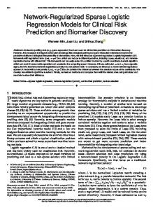
Discussion of experimental results Figure 1 shows the results for the five algorithms specifically designed for L1 regularized logistic regression (IRLSLARS, Grafting, SCGIS, GenLASSO and Gl1ce) on 12 datasets. Since the running times for the standard optimization methods (CG-L1, NM-epsL1, CG-epsL1 and CGHuber) tend to be significantly higher, we do not report them in the same figure. (Doing so allows us to visualize more clearly the differences in performance for the first set of algorithms.) We report the performance of the standard optimization algorithms (and our algorithm) in Table 3. In all cases we report the average running time (in seconds) over 100 trials of the same experiment (dataset and algorithm combination). The results reported in Figure 1 show that our algorithm (IRLS-LARS) was more efficient than all other algorithms in 11 out of 12 datasets. On one dataset (Microarray2) GenLasso and Gl1ce were slightly faster. All other algorithms were slower than our algorithm on every dataset. IRLS-LARS significantly outperformed Grafting and SCGIS. More specifically, in 8 (out of 12) datasets our method was more than 8 times faster than Grafting. (In the other 4, it was also faster, although not by a factor of 8.) Our method was at least 10 times faster than SCGIS in 10 out of 12 datasets. GenLASSO and Gl1ce are the strongest competitors, and even then our algorithm is more than twice as fast as Gl1ce 8 In all cases, the primal constraint (kθk1 ≤ C) was satisfied with an error less than 10−13 , and Equation (24) was satisfied with an error less than 5 × 10−8 . All the other KKT conditions were satisfied exactly. We performed the same procedure using GenLASSO and obtained similar results. In all cases, the absolute difference between the obj ∗ ’s obtained from running IRLS-LARS and the obj ∗ ’s obtained from running GenLASSO was smaller than 10−8 ; and the relative difference was always smaller than 10−10 .

Data Arrhythmia Hepatitis Ionosphere Promoters Spambase Spect Spectf Splice WBCa Madelon Microarray1 Microarray2 a

IRLSLARS 0.0420 0.0046 0.0516 0.0182 4.0804 0.0345 0.0646 0.8376 0.1222 0.8602 0.0330 0.4069

NMepsL1 2.8450 0.0258 0.1534 0.0632 21.172 0.0704 0.2330 2.9828 0.7225 55.060 242.88 500.00

CGepsL1 14.384 0.0819 0.1746 0.2047 10.151 0.1206 0.5493 0.9424 4.9592 113.22 500.00 500.00

CGHuber 13.660 0.6580 0.9717 0.8418 13.410 0.7651 1.1761 4.3407 1.4854 95.223 500.00 500.00

CGL1 14.065 0.6347 0.9237 0.7328 12.016 0.7293 1.1235 4.8007 1.3777 104.50 500.00 500.00

Wisconsin breast cancer

Table 3: The running time (seconds) of IRLS-LARS, CG-L1 and three algorithms with the approximate L1 functions (NM-epsL1, CG-epsL1 and CG-Huber). (See text for details.)

for 5 out of 12 datasets and more than twice as fast as GenLASSO for 8 out of 12 datasets. We note that (as opposed to ours and all the other methods) GenLASSO is highlyoptimized C code (linked with highly optimized numerical libraries). It is widely accepted that C code is faster than MATLAB code, and thus we are giving GenLASSO a somewhat unfair advantage in our comparison.9 As reported in Table 3, conjugate gradient and Newton’s method are an order of magnitude slower than our IRLSLARS algorithm in most of the datasets (despite the less stringent stopping criterion). Among these methods, NMepsL1 seems to be the second best algorithm on the datasets with a small number of features. However, this method quickly becomes inefficient as the number of features increases. Also other methods similarly suffered from the increasing number of features. We observe that CG-L1 is very competitive with CG-epsL1 and CG-Huber.

Conclusions In this paper, we proposed a new algorithm for learning L1 regularized logistic regression. Our theoretical results show that our algorithm is guaranteed to converge to a global optimum. Our experiments showed that our algorithm is computationally very efficient. In particular, it outperforms standard algorithms for solving convex optimization problems, as well as other algorithms previously developed specifically to solve the L1 regularized logistic regression problem. 9

We have implemented GenLASSO in MATLAB. However, the extensive optimization tricks used in the C-code and numerical libraries were hard to be duplicated in MATLAB, making it hard to evaluate GenLASSO correctly with our MATLAB code. Since C code is widely accepted to be at least as fast as MATLAB code, we decided to report the C code results (possibly favoring GenLASSO somewhat in our comparisons).

Acknowledgments We give warm thanks to John Lafferty, Alexis Battle, Ben Packer, and Vivek Farias for helpful comments. H. Lee was supported by Stanford Graduate Fellowship (SGF). This work was supported in part by the Department of the Interior/DARPA under contract number NBCHD030010.

References Boyd, S., and Vandenberghe, L. 2004. Convex Optimization. Cambridge University Press. Efron, B.; Hastie, T.; Johnstone, I.; and Tibshirani, R. 2004. Least angle regression. Annals of Statistics 32(2):407–499. Goodman, J. 2004. Exponential priors for maximum entropy models. In Proceedings of the Annual Meeting of the Association for Computational Linguistics. Green, P. J. 1984. Iteratively reweighted least squares for maximum likelihood estimation, and some robust and resistant alternatives. Journal of the Royal Statistical Society, Series B, Methodological 46:149–192. Lokhorst, J. 1999. The LASSO and Generalised Linear Models. Honors Project, Department of Statistics, The University of Adelaide, South Australia, Australia. McCullagh, P., and Nelder, J. A. 1989. Generalized Linear Models. Chapman & Hall. Minka, T. P. 2003. A comparison of numerical optimizers for logistic regression. http://research. microsoft.com/˜minka/papers/logreg/. Nelder, J. A., and Wedderbum, R. W. M. 1972. Generalized linear models. Journal of the Royal Statistical Society, Series A, General 135(3):370–384. Newman, D. J.; Hettich, S.; Blake, C. L.; and Merz, C. 1998. UCI repository of machine learning databases. http://www.ics.uci.edu/˜mlearn/ MLRepository.html. Ng, A. Y. 2004. Feature selection, l1 vs. l2 regularization, and rotational invariance. In International Conference on Machine Learning. Osborne, M.; Presnell, B.; and Turlach, B. 2000. On the lasso and its dual. Journal of Computational and Graphical Statistics 9:319–337. Perkins, S., and Theiler, J. 2003. Online feature selection using grafting. In International Conference on Machine Learning. Rockafellar, R. T. 1970. Convex analysis. Princeton Univ. Press. Roth, V. 2004. The generalized lasso. IEEE Trans. Neural Networks 15(1):16–28. Royden, H. 1988. Real Analysis. Prentice Hall. Tibshirani, R. 1996. Regression shrinkage and selection via the lasso. Journal of the Royal Statistical Society, Series B 58(1):267–288.

Figure 1: Comparison of the running time (seconds) among five algorithms (IRLS-LARS, Grafting, SCGIS, GenLASSO and Gl1ce) over 12 datasets. Each plot corresponds to one dataset. The name of the dataset is indicated at the top of the plot, and the number of features (N ) and the number of training instances (M ) are shown as “Name of the data: N × M ”. For each experiment, we report the running time in seconds, and the running time relative to IRLS-LARS in parentheses. (See text for discussion.)