The increase in the number of video copies, both legal and illegal, has become a major problem in the multime- dia and I
Fast Min-hashing Indexing and Robust Spatiotemporal Matching for Detecting Video Copies CHIH-YI CHIU, National Chiayi University HSIN-MIN WANG, AND CHU-SONG CHEN Institute of Information Science, Academia Sinica ________________________________________________________________________ The increase in the number of video copies, both legal and illegal, has become a major problem in the multimedia and Internet era. In this paper, we propose a novel method for detecting various video copies in a video sequence. To achieve fast and robust detection, the method fully integrates several components, namely the min-hashing signature to compactly represent a video sequence, the spatio-temporal matching scheme to accurately evaluate the video similarity compiled from the spatial and temporal aspects, and some speed-up techniques to expedite both min-hashing indexing and spatio-temporal matching. The results of experiments demonstrate that, compared to several baseline methods with different feature descriptors and matching schemes, the proposed method that combines both global and local feature descriptors yields the best performance when encountering a variety of video transformation. The method is very fast, requiring approximately 0.06 seconds to search for copies of a thirty-second video clip in a six-hour video sequence. Categories and Subject Descriptors: H.3.3 [Information Storage and Retrieval]: Information Search and Retrieval - Information filtering, Search process; I.2.10 [Artificial Intelligence]: Vision and Scene Understanding - Video analysis General Terms: Algorithms, Design, Experimentation, Performance Additional Key Words and Phrases: Content-based copy detection, near-duplicate, histogram pruning
________________________________________________________________________ 1. INTRODUCTION With the rapid development of multimedia technologies, digital videos are now ubiquitous on the Internet. According to a report by AccuStream iMedia Research (http://www.accustreamresearch.com), in 2006, the quantity of video streams increased 38.8% to 24.92 billion in media sites world-wide. One of the most popular video sharing sites, YouTube, hosted about 6.1 million videos, and 65,000 video clips were uploaded everyday. The enormous growth in the amount of video data has led to the requirement for efficient and effective techniques of video indexing and retrieval. In particular, since digital videos can be easily duplicated, edited, and disseminated, video copying has become an increasingly serious problem. A video copy detection technique would thus be helpful for protecting and managing video content. For instance, with such a technique, content providers could track particular videos with respect to royalty payments and Some parts of this work were published in Chiu et al. [2007]. This work was supported in part by the National Science Council of Taiwan under Grants NSC 98-2218-E-415003 and NSC 99-2631-H-001-020. Authors' addresses: C. Y. Chiu, National Chiayi University; email:
[email protected]; H. M. Wang, and C. S. Chen: Institute of Information Science, Academia Sinica, 128 Academia Road, Section 2, Nankang, Taipei 115, Taiwan. © 2008 ACM 1073-0516/01/0300-0034 $5.00
1
possible copyright infringements. Platform providers could remove identical copies uploaded by users or aggregate near-duplicate videos into groups to facilitate browsing. Fig. 1 shows the result of inputting the phrase "UFO Apollo 11" to YouTube. Several sets of identical or near-duplicate video clips are displayed on the search result page. If the nearduplicates of the same set are compacted into a single item, the search result page can display more diverse video clips for users.
Fig. 1. The first fourteen search results retrieved by inputting the phrase "UFO Apollo 11" to YouTube. Most of the video clips are identical or near-duplicates, which can be removed or aggregated to facilitate user browsing.
There are two general techniques for detecting video copies: digital watermarking and content-based copy detection. Digital watermarking embeds hidden information in video, while the content-based technique employs perceptual features of the video content as a unique signature to distinguish one video from another. Because the latter does not destroy or damage video content, it has generated a great deal of research interest recently. Most existing content-based methods treat a video as a set of individual image frames and focus on the investigation of compact image features or efficient index structures. However, this confines their use to particular applications. For example, some methods are limited to dealing with certain types of video transformation, while others are limited to other types depending on the properties of the features they use. Besides, since these methods seldom consider time-related features, they have difficulty handling video transformation types that modify the temporal structure of video, such as slow motion and frame insertion/deletion. The pre-built index structures also cause an inherent search limitation, as some methods need to partition a video sequence into basic index units (e.g., shots) in advance. These methods might be inappropriate for monitoring broadcast streams. In this paper, we address the limitations posed by existing methods. We classify various video copies into four categories with respect to the spatial and temporal transformation. While current methods are limited to handling one or two categories, we propose a novel video content analysis scheme, called spatio-temporal matching, to tackle all the
2
categories in a unified manner. The proposed matching scheme, which analyzes the content similarity of two videos compiled from the spatial and temporal aspects, can effectively handle a variety of video transformation. To avoid the limitation caused by the pre-built index structures, we employ a sliding window approach that would be more appropriate for monitoring broadcast streams. Without the index structures, however, the search time spent on a large-scale video sequence would be considerable. To make the search more efficient, the proposed method adopts a coarse-to-fine matching strategy. In the coarse stage, the sliding window scans the entire sequence to find potential candidate clips quickly. Each windowed sequence, as well as the given query clip, is represented by a novel feature called the min-hashing signature that is compact and robust. For example, in this study, a 30-dimensional signature is sufficient to represent a sixty-frame sequence. In the fine stage, the above-mentioned spatio-temporal matching is used to filter out false positives from the candidate set. In addition, some speed-up techniques are applied in both stages with great effect; hence, overall, the proposed method is very fast. To evaluate the proposed method, we implement several baseline methods that use different feature descriptors (e.g., the ordinal measure and the SIFT descriptor), as well as different matching schemes. The results of extensive experiments show that, with the composed feature descriptor, the proposed method achieves excellent results, which demonstrate the widest coverage for various transformation types among all compared methods. The proposed method is also very efficient, as it only needs about 0.06 seconds to search for copies of a thirty-second query clip in a six-hour video sequence. The remainder of this paper is organized as follows. In Section 2, we formulate the video copy detection problem. Section 3 reviews recent work related to video copy detection. In Section 4, we detail the proposed method, including min-hashing indexing and spatio-temporal matching. Section 5 describes the extensive evaluation experiments. Then, in Section 6, we summarize our conclusions.
2. PROBLEM FORMULATION Let Q be a query clip with n frames, and T be a target sequence with m frames, where n 0 , qi is inserted into the l-th cell of IT. We apply the same step to insert every candidate frame cp into the corresponding cells of IT. Then, we construct PM by scanning IT as follows: for each frame pair (qi, cp) found in the l-th cell of IT, we update the (i, p)-th element mip of PM by adding min(qhl( i ) , chl( p ) ) . When only a few frame pairs intersect in some histogram bins, using the inverted table can reduce the computation cost substantially. The computation time mainly comprises of inserting frames into IT and accumulating the number of frame pairs in IT. Further discussions are given in experiments. 15
5. EXPERIMENTS
To evaluate the proposed method, we compiled a video dataset for use in several experiments. The code was implemented in C++, and the evaluation was carried out on a PC with a 1.8 GHz CPU and 2GB RAM.
5.1. Video Dataset
A 6.1-hour video sequence was compiled from the MPEG-7 video CD collection and the Open Video Project (http://www.open-video.org/). Its contents included sports programs, news broadcasts, and documentaries. We transformed these video data into the following uniform format: MPEG-1, 320×240 pixels, and 30 frames per second (fps). This dataset served as the target sequence. From the target sequence, we randomly extracted 31 subsequences, each of 30 seconds duration. Each subsequence derived twelve video copies by applying the common video transformation types listed in Table 1. Fig. 7 gives two examples of frame orderchanged temporal transformation used in the experiments. There were totally 372 (31×12) video copies, which served as the query clips. Each copy was used to detect the corresponding subsequence in the target sequence. Note that the definition of the target sequence and query clips here is different from that given in Section 2. We made this modification to fit the experiment's purpose; that is, to only generate a small size of the query dataset. Since a continuous video sequence contains many identical or near-duplicate frames, it is not necessary to use every frame in the sequence for matching. Therefore, we selected a key frame every 15 frames of the target sequence. In other words, the frame rate of the target sequence became 2 fps. In addition, before starting the detection process, we had to determine the frame rate of the query clip, which is commonly available from the file header. The query clip was re-sampled so that its frame rate is synchronized with that of the target sequence. For example, a 30-second query clip with 30fps became a 60frame sequence after re-sampling.
Table 1. Different types of video transformation. Category
Type
Description
Whole region-preserved
Brightness
Enhance the brightness by 20%.
spatial transformation
Compression
Set the compression quality 50% (by IndeoR 5.10).
Noise
Add 10% random noise.
16
Equalization
Equalize the color histogram.
Resolution change
Change the frame resolution to 120×90 pixels.
Partial region-discarded
Cropping
Crop the top and bottom frame regions by 10% each.
spatial transformation
Zooming in
Zoom in to the frame by 10%.
Frame number-changed
Slow motion
Halve the video speed.
temporal transformation
Fast forward
Double the video speed.
Frame rate change
Change the frame rate to 15 fps.
Frame order-changed
Swap
Swap the first-half subsequence and the second-half one.
temporal transformation
Insertion/deletion
Delete middle 50% of frames and insert unrelated frames.
(a)
(b)
Fig. 7. Examples of frame order-changed temporal transformation used in the experiments: (a) Swap the firsthalf subsequence and the second-half one. (b) Delete middle 50% of frames and insert unrelated frames.
5.2 Feature Extraction
From each frame, we extracted the ordinal measure and the SIFT descriptor to serve as the global descriptor and local descriptor, respectively. To extract the ordinal measure, we partitioned each video frame into Nx×Ny non-overlapping blocks and computed their intensity ranks. The rank order is known as the ordinal measure of the frame. Since there were (Nx×Ny)! possible permutations of the ordinal measure, we used a histogram with (Nx×Ny)! bins to represent a video sequence, where each frame was assigned to a histogram bin according to its ordinal measure. Here Nx = 3 and Ny = 2. To extract SIFT descriptors of each frame, we located the local extrema in the DOG (Differential-of-Gaussian) scale space and computed their orientation histograms in the image space. We used a training dataset collected from another video collection, and applied the LBG (Linde-Buzo-Gray) algorithm [Sayood 1996] to generate a codebook of L codewords. Then, each SIFT descriptor was quantized to the nearest codeword and assigned to the corresponding histogram bin. Subsequently, a video sequence was represented by a histogram with L bins. Here L = 1024. For every frame, we extracted one ordinal measure and averagely 22.84 SIFT descriptors in this dataset. As mentioned earlier, the ordinal measure and the SIFT descriptor can be combined to improve the accuracy. To this end, we simply executed the search twice using the ordinal measure and the SIFT descriptor individually to collect their corresponding candidate sets, which were then merged into a single one. For a candidate sequence in the merged set,
17
let PMordinal and PMSIFT be the pairwise matrixes generated based on ordinal measure and SIFT descriptor, respectively; and let PMcombination be the combined form written as: PMcombination = α ⋅ PMordinal + (1-α) ⋅ PMSIFT ,
(10)
where α ∈ [0, 1] is a weighting factor that controls the relative importance of PMordinal and PMSIFT. We set α = 0.5 throughout the experiments. 5.3 Evaluation Metric
We used the following detection criteria for the accuracy evaluation. A detection result was considered correct if it had any overlap with the region from which the query was extracted. The recall and precision rates were used to evaluate the accuracy of the detection result: recall = TP / (TP + FN),
(11)
precision = TP / (TP + FP),
(12)
where True Positives (TP) refer to positive examples correctly labeled as positives; False Negatives (FN) refer to positive examples incorrectly labeled as negatives; and False Positives (FP) refer to negative examples incorrectly labeled as positives. We also used the F-measure, calculated as: F-measure = (2×recall×precision) / (recall + precision).
(13)
5.4 Overview of Methods Evaluated
We implemented the following seven methods for performance evaluation: (1) The ordinal measure with spatio-temporal matching (abbreviated as "OM+STM"). (2) The SIFT descriptor with spatio-temporal matching ("SD+STM"). (3) The combination of Methods (1) and (2) using Equation (10) ("OM+SD+STM"). (4) The ordinal measure without spatio-temporal matching ("OM"). (5) The SIFT descriptor without spatio-temporal matching ("SD"). (6) Method (2) without min-hashing ("SD+STM-MH"). (7) Hoad and Zobel's method [2006] ("HZ").
Methods (1) and (2) used different min-hashing features with spatio-temporal matching, and their combination yielded Method (3). We implemented Methods (4) and (5) to see the effect without the proposed spatio-temporal matching scheme. Method (6) was implemented to assess the proposed min-hashing indexing. The threshold parameters used in Methods (1)-(5) were configured as follows. For min-hashing similarity computation, we set θMS = 0.5; for spatio-temporal matching, we set θEM = G/4, where G is the 18
maximum among all edge magnitudes in the pairwise matrix, ΘED = [20°, 70°], and θLM = n/5. In Method (6), the Jaccard similarity threshold θJS was adjusted to control the trade-off between the recall and precision rates. We finally set θJS = 0.35 since its accuracy was closest to that of Method (2) in several transformation types. We can thus compare the computation cost of Method (2) and Method (6) (with min-hashing indexing vs. without min-hashing indexing). In Method (7), the recall and precision rates were measured after x results were detected, where x is the number of positives (video copies) in the target sequence. Recall that k and g are the min-hashing signature lengths of a sequence and a frame, respectively. The configurations of the (k, g) pairs were set according to the feature used. For the methods using the SIFT descriptor, i.e., Methods (2) and (5), we used the following ten empirical (k, g) pairs in the experiments: (10, 2), (20, 3), (30, 3), (40, 3), (50, 4), (60, 4), (70, 5), (80, 5), (90, 6), and (100, 6). For the methods using the ordinal measure, i.e., Methods (1) and (4), each frame had only one ordinal measure; hence, g was always set to 1. In Method (3), which combines the ordinal measure and SIFT descriptor, we used the above ten (k, g) pairs for the SIFT descriptor part and the pair (k, g) = (30, 1) for the ordinal measure part. Methods (6) and (7) did not involve k and g. Hoad and Zobel's method, i.e., Method (7), is one of the state of the art methods that use the window sliding approach. We implemented their method as follows. In each frame, the color-shift signature was extracted by using 16 bins for each of the three color channels in YCbCr. The Manhattan distance was used to calculate the histogram distance of two adjacent frames. To extract the centroid-based signature, we identified the lightest and darkest 5% of pixels in each frame, and computed their average coordinates as the centroid location. We calculated the Euclidean distance of the centroids between two adjacent frames. The two distance signatures were combined into a single vector to represent a frame, and approximate string matching was applied for similarity measurement. This method can provide a perspective on the typical window sliding approach using a global descriptor.
5.5 Detection Accuracy
In the following subsections, we show and discuss the accuracy of the compared methods in terms of spatial and temporal transformation.
5.5.1 Whole region-preserved spatial transformation. This category includes brightness enhancement, compression, noise addition, histogram equalization, and frame reso19
lution change, which have been widely tested by existing methods. The results are listed in Tables 2-6. The bold font indicates the highest F-measure scores in the table. The length of the min-hashing signature has quite a large impact on the retrieval accuracy of the ordinal-based methods (i.e., Methods (1) and (4)). The recall rate degrades and the precision rate improves as k grows to 60. Since the query clip contains 60 frames after re-sampling, the maximum length of the ordinal-based min-hashing signature is 60. This explains why the performance will not change when k > 60. In contrast, the length of the min-hashing signature has a limited impact in the SIFT-based methods (i.e., Methods (2) and (5)), with slight variations in the recall and precision rates under various k. The performance of the SIFT-based methods is superior to that of the ordinal-based methods for the brightness, compression, and noise transformation types. However, for the equalization and resolution change types, the recall rates of the SIFT-based methods decline sharply. This is because applying the two transformation types might alter the original SIFT descriptor's property substantially. Compared with the SIFT-based methods, the ordinal-based methods yield nearly similar results for all types of whole regionpreserved spatial transformation. With a suitable choice of k, the ordinal-based methods would gain a more robust performance than the SIFT-based methods in this transformation category. The proposed spatio-temporal matching scheme is effective in improving the precision rates of both ordinal-based and SIFT-based methods. In particular for the SIFTbased methods, Method (2) obtains a substantial improvement from Method (5). From another perspective, Method (5) retrieves a large number of false positives, while Method (2) utilizes the proposed matching scheme to remove these false positives effectively. Method (6) obtains extremely good results for the brightness, compression, and noise transformation types. Its accuracy served as an upper bound for Method (2) in these transformation types. From Tables 2-6, we observe that the gap is not very significant. Hoad and Zobel's method, i.e., Method (7), performs well for the compression, noise, and resolution change types, but not as well for the brightness and equalization types. This is because its color-shift signature counts the histograms of the color channels that might vary widely after applying brightness enhancement or histogram equalization. Among all the methods, Method (3), i.e., the combination of Methods (1) and (2), yields the most robust results in all types of whole region-preserved spatial transformation. Method (3) exhibits a similar accuracy distribution to that of Method (2); however, because of the combination of the ordinal measure and SIFT descriptor, the accuracy distribution of Method (3) is more compact and expresses better precision and recall rates. 20
Table 2. The precision and recall rates for brightness transformation. (1) OM+STM (2) SD+STM (3) OM+SD+STM (4) OM (5) SD (6) SD+STM-MH (7) HZ
R P R P R P R P R P R P R P
k=10 1.0000 0.3523 0.9032 0.9333 1.0000 0.9394 1.0000 0.1348 1.0000 0.0110 1.0000 1.0000 0.7742 0.7742
k=20 0.9355 0.6591 0.9677 0.9375 1.0000 0.9394 0.9355 0.5686 0.9677 0.0258 1.0000 1.0000 0.7742 0.7742
k=30 0.9355 0.8529 0.9677 0.9091 1.0000 0.9118 0.9355 0.8056 0.9677 0.0296 1.0000 1.0000 0.7742 0.7742
k=40 0.7419 1.0000 1.0000 0.9394 1.0000 0.9394 0.7419 0.9583 1.0000 0.0546 1.0000 1.0000 0.7742 0.7742
k=50 0.5806 1.0000 0.9677 0.9375 1.0000 0.9394 0.5806 1.0000 0.9677 0.0571 1.0000 1.0000 0.7742 0.7742
k=60 0.2258 1.0000 0.9677 0.9677 1.0000 0.9688 0.2258 1.0000 0.9677 0.0993 1.0000 1.0000 0.7742 0.7742
k=70 0.2258 1.0000 0.9677 0.9677 1.0000 0.9688 0.2258 1.0000 0.9677 0.0962 1.0000 1.0000 0.7742 0.7742
k=80 0.2258 1.0000 0.9355 0.9677 1.0000 0.9688 0.2258 1.0000 0.9355 0.1312 1.0000 1.0000 0.7742 0.7742
k=90 0.2258 1.0000 0.9355 0.9677 1.0000 0.9688 0.2258 1.0000 0.9355 0.1394 1.0000 1.0000 0.7742 0.7742
k=100 0.2258 1.0000 0.9355 0.9677 1.0000 0.9688 0.2258 1.0000 0.9355 0.1648 1.0000 1.0000 0.7742 0.7742
Table 3. The precision and recall rates for compression transformation. (1) OM+STM (2) SD+STM (3) OM+SD+STM (4) OM (5) SD (6) SD+STM-MH (7) HZ
R P R P R P R P R P R P R P
k=10 1.0000 0.3483 0.8387 0.9286 1.0000 0.9118 1.0000 0.1360 0.9032 0.0103 0.9677 1.0000 0.9355 0.9355
k=20 0.9355 0.6304 0.8710 0.9310 0.9355 0.9355 0.9355 0.5577 0.9032 0.0223 0.9677 1.0000 0.9355 0.9355
k=30 0.9355 0.8529 0.9677 0.9677 0.9677 0.9677 0.9355 0.8056 1.0000 0.0262 0.9677 1.0000 0.9355 0.9355
k=40 0.7742 0.9231 0.9677 0.9677 0.9677 0.9677 0.7742 0.9231 1.0000 0.0458 0.9677 1.0000 0.9355 0.9355
k=50 0.6129 0.9500 0.9355 0.9355 0.9677 0.9677 0.6129 0.9500 0.9667 0.0439 0.9677 1.0000 0.9355 0.9355
k=60 0.2581 1.0000 0.9355 0.9667 0.9677 0.9375 0.2581 1.0000 0.9667 0.0699 0.9677 1.0000 0.9355 0.9355
k=70 0.2581 1.0000 0.9355 0.9667 0.9677 0.9677 0.2581 1.0000 0.9667 0.0699 0.9677 1.0000 0.9355 0.9355
k=80 0.2581 1.0000 0.9355 0.9667 1.0000 0.9688 0.2581 1.0000 0.9355 0.0945 0.9677 1.0000 0.9355 0.9355
k=90 0.2581 1.0000 0.8710 0.9643 0.9677 0.9677 0.2581 1.0000 0.9032 0.0930 0.9677 1.0000 0.9355 0.9355
k=100 0.2581 1.0000 0.8710 0.9643 0.9677 0.9677 0.2581 1.0000 0.9032 0.1197 0.9677 1.0000 0.9355 0.9355
k=90 0.2258 1.0000 0.8387 0.9286 1.0000 0.9394 0.2258 1.0000 0.9032 0.0824 1.0000 1.0000 0.9032 0.9032
k=100 0.2258 1.0000 0.8710 0.9310 1.0000 0.9394 0.2258 1.0000 0.9032 0.1089 1.0000 1.0000 0.9032 0.9032
Table 4. The precision and recall rates for noise transformation. (1) OM+STM (2) SD+STM (3) OM+SD+STM (4) OM (5) SD (6) SD+STM-MH (7) HZ
R P R P R P R P R P R P R P
k=10 1.0000 0.3605 0.8065 0.8929 1.0000 0.9118 1.0000 0.1396 0.8387 0.0089 1.0000 1.0000 0.9032 0.9032
k=20 0.9355 0.6905 0.8065 0.8065 1.0000 0.8378 0.9355 0.6304 0.8387 0.0185 1.0000 1.0000 0.9032 0.9032
k=30 0.9355 0.9063 0.9355 0.8286 1.0000 0.8378 0.9355 0.8529 0.9355 0.0221 1.0000 1.0000 0.9032 0.9032
k=40 0.7419 1.0000 0.9677 0.8824 1.0000 0.8857 0.7419 0.9583 0.9677 0.0384 1.0000 1.0000 0.9032 0.9032
k=50 0.5806 1.0000 0.8710 0.9310 1.0000 0.9394 0.5806 1.0000 0.9355 0.0389 1.0000 1.0000 0.9032 0.9032
k=60 0.2258 1.0000 0.9032 0.9032 1.0000 0.9118 0.2258 1.0000 0.9355 0.0556 1.0000 1.0000 0.9032 0.9032
k=70 0.2258 1.0000 0.9032 0.9032 1.0000 0.9118 0.2258 1.0000 0.9355 0.0577 1.0000 1.0000 0.9032 0.9032
k=80 0.2258 1.0000 0.8710 0.9310 1.0000 0.9394 0.2258 1.0000 0.9355 0.0788 1.0000 1.0000 0.9032 0.9032
Table 5. The precision and recall rates for equalization transformation. (1) OM+STM (2) SD+STM (3) OM+SD+STM (4) OM
R P R P R P R P
k=10 0.8387 0.2766 0.2903 0.6429 0.8065 0.8333 0.9355 0.1184
k=20 0.9032 0.6829 0.3548 0.7333 0.8065 0.8621 0.9032 0.6222
k=30 0.8387 0.8667 0.3548 0.7857 0.8065 0.8929 0.8387 0.8125
k=40 0.4194 1.0000 0.3226 0.8333 0.7742 0.9231 0.4194 1.0000
21
k=50 0.2581 1.0000 0.2581 1.0000 0.7419 1.0000 0.2581 1.0000
k=60 0.0323 1.0000 0.3226 0.9091 0.7419 0.9583 0.0323 1.0000
k=70 0.0323 1.0000 0.2903 0.9000 0.7419 0.9583 0.0323 1.0000
k=80 0.0323 1.0000 0.1935 0.8571 0.7419 0.9583 0.0323 1.0000
k=90 0.0323 1.0000 0.1613 0.8333 0.7419 0.9583 0.0323 1.0000
k=100 0.0323 1.0000 0.1613 0.8333 0.7419 0.9583 0.0323 1.0000
(5) SD (6) SD+STM-MH (7) HZ
R P R P R P
0.5161 0.0071 0.2258 1.0000 0.5806 0.5806
0.4839 0.0164 0.2258 1.0000 0.5806 0.5806
0.5484 0.0217 0.2258 1.0000 0.5806 0.5806
0.5161 0.0430 0.2258 1.0000 0.5806 0.5806
0.3871 0.0399 0.2258 1.0000 0.5806 0.5806
0.3871 0.0833 0.2258 1.0000 0.5806 0.5806
0.3871 0.0764 0.2258 1.0000 0.5806 0.5806
0.2903 0.1098 0.2258 1.0000 0.5806 0.5806
0.2258 0.1167 0.2258 1.0000 0.5806 0.5806
0.2258 0.2121 0.2258 1.0000 0.5806 0.5806
Table 6. The precision and recall rates for resolution change transformation. (1) OM+STM (2) SD+STM (3) OM+SD+STM (4) OM (5) SD (6) SD+STM-MH (7) HZ
R P R P R P R P R P R P R P
k=10 1.0000 0.3229 0.5484 0.8947 0.9032 0.9032 1.0000 0.1225 0.6774 0.0085 0.5806 1.0000 0.8710 0.8710
k=20 0.9355 0.6042 0.4839 0.9375 0.9032 0.9655 0.9355 0.5472 0.7097 0.0199 0.5806 1.0000 0.8710 0.8710
k=30 0.9355 0.7436 0.5484 0.9444 0.9032 0.9655 0.9355 0.6905 0.7419 0.0237 0.5806 1.0000 0.8710 0.8710
k=40 0.7419 1.0000 0.6129 0.9048 0.9677 0.9375 0.7419 0.9583 0.7742 0.0519 0.5806 1.0000 0.8710 0.8710
k=50 0.5806 1.0000 0.6452 0.9091 0.9355 0.9063 0.5806 1.0000 0.7419 0.0535 0.5806 1.0000 0.8710 0.8710
k=60 0.2581 1.0000 0.6129 0.8636 0.9355 0.9063 0.2581 1.0000 0.6452 0.0794 0.5806 1.0000 0.8710 0.8710
k=70 0.2581 1.0000 0.5806 0.9474 0.9355 0.9355 0.2581 1.0000 0.6452 0.0680 0.5806 1.0000 0.8710 0.8710
k=80 0.2581 1.0000 0.5806 0.9000 0.9355 0.9063 0.2581 1.0000 0.6452 0.1005 0.5806 1.0000 0.8710 0.8710
k=90 0.2581 1.0000 0.6129 0.9048 0.9355 0.9355 0.2581 1.0000 0.6452 0.0990 0.5806 1.0000 0.8710 0.8710
k=100 0.2581 1.0000 0.6129 0.9048 0.9355 0.9355 0.2581 1.0000 0.6774 0.1214 0.5806 1.0000 0.8710 0.8710
5.5.2 Partial region-discarded spatial transformation. This category includes cropping and zooming in. The results are shown in Tables 7 and 8. For the ordinal-based methods, the recall rates degrade slightly in both the cropping and zooming in types. Moreover, their performances in partial region-discarded spatial transformation are not as good as those in whole region-preserved spatial transformation. This is because a frame's ordinal measure, which models the property of the whole frame region, might be totally different if the frame is modified by partial region-discarded spatial transformation. The same problem arises in Hoad and Zobel's method because its signature also models the whole frame region property. Interestingly, Hoad and Zoble's method performs poorly in the cropping type, but quite well in the zooming in type. On the other hand, the SIFT descriptor is less affected in this transformation category. Actually, Method (2) achieves good results. Although the ordinal measure and the SIFT descriptor have both advantages and limitations, their different characteristics complement each other very well. Combining the two features not only enhances the detection accuracy, but also widens the coverage to more transformation types. Method (3) provides good evidence to support the above viewpoint.
Table 7. The precision and recall rates for cropping transformation. (1) OM+STM (2) SD+STM (3) OM+SD+STM
R P R P R P
k=10 0.6774 0.2838 0.8387 0.9630 0.9355 0.9667
k=20 0.7742 0.5455 0.8387 0.8966 0.9355 0.9063
k=30 0.6774 0.8400 0.8065 0.8929 0.9355 0.9063
k=40 0.2258 1.0000 0.8387 0.8966 0.9032 0.9032
22
k=50 0.0968 1.0000 0.8710 0.9000 0.9355 0.9063
k=60 0.0323 1.0000 0.8710 0.9310 0.9032 0.9333
k=70 0.0323 1.0000 0.8710 0.9310 0.9032 0.9333
k=80 0.0323 1.0000 0.8387 0.9630 0.9032 0.9655
k=90 0.0323 1.0000 0.8387 0.9630 0.9032 0.9655
k=100 0.0323 1.0000 0.8387 0.9630 0.9032 0.9655
(4) OM (5) SD (6) SD+STM-MH (7) HZ
R P R P R P R P
0.7097 0.1053 0.9032 0.0088 0.8065 1.0000 0.2903 0.2903
0.7742 0.4211 0.8710 0.0190 0.8065 1.0000 0.2903 0.2903
0.7097 0.8148 0.8710 0.0207 0.8065 1.0000 0.2903 0.2903
0.2258 1.0000 0.8710 0.0356 0.8065 1.0000 0.2903 0.2903
0.0968 1.0000 0.9032 0.0393 0.8065 1.0000 0.2903 0.2903
0.0323 1.0000 0.9032 0.0625 0.8065 1.0000 0.2903 0.2903
0.0323 1.0000 0.9032 0.0606 0.8065 1.0000 0.2903 0.2903
0.0323 1.0000 0.8710 0.0836 0.8065 1.0000 0.2903 0.2903
0.0323 1.0000 0.8710 0.0925 0.8065 1.0000 0.2903 0.2903
0.0323 1.0000 0.8710 0.1084 0.8065 1.0000 0.2903 0.2903
Table 8. The precision and recall rates for zooming in transformation. (1) OM+STM (2) SD+STM (3) OM+SD+STM (4) OM (5) SD (6) SD+STM-MH (7) HZ
R P R P R P R P R P R P R P
k=10 0.6129 0.2375 0.6129 0.8636 0.8065 0.8929 0.7097 0.0873 0.8065 0.0104 0.6452 1.0000 0.8710 0.8710
k=20 0.7742 0.5714 0.8065 0.9259 0.9355 0.9355 0.8065 0.4630 0.8387 0.0250 0.6452 1.0000 0.8710 0.8710
k=30 0.6452 0.8333 0.8710 0.9000 0.9355 0.9063 0.6774 0.7500 0.9355 0.0287 0.6452 1.0000 0.8710 0.8710
k=40 0.3226 1.0000 0.8065 0.9259 0.9355 0.9355 0.3226 1.0000 0.8387 0.0466 0.6452 1.0000 0.8710 0.8710
k=50 0.1290 1.0000 0.8387 0.9286 0.9355 0.9355 0.1290 1.0000 0.9032 0.0535 0.6452 1.0000 0.8710 0.8710
k=60 0.0323 1.0000 0.8387 0.9630 0.9355 0.9667 0.0323 1.0000 0.8710 0.0918 0.6452 1.0000 0.8710 0.8710
k=70 0.0323 1.0000 0.8710 0.9310 0.9355 0.9355 0.0323 1.0000 0.9032 0.0915 0.6452 1.0000 0.8710 0.8710
k=80 0.0323 1.0000 0.8387 0.9630 0.9032 0.9655 0.0323 1.0000 0.8387 0.1171 0.6452 1.0000 0.8710 0.8710
k=90 0.0323 1.0000 0.8065 0.9615 0.9032 0.9655 0.0323 1.0000 0.8065 0.1283 0.6452 1.0000 0.8710 0.8710
k=100 0.0323 1.0000 0.8065 0.9615 0.8710 0.9643 0.0323 1.0000 0.8065 0.1397 0.6452 1.0000 0.8710 0.8710
5.5.3 Frame number-changed temporal transformation. This category includes slow motion, fast forward, and frame rate change. The results are shown in Tables 9-11. The slow motion and fast forward types halve and double the query video speed, respectively; thus, a 30-second source sequence becomes 60-second query clip and 15second query clip, respectively. The change in the query video's speed induces that the query content does not synchronize with the target content in the window. For the frame rate change type, Methods (1)-(6) re-sample each query video to synchronize with the target sequence's frame rate, whereas Method (7) matches the two sequence frames directly without re-sampling. In the slow motion and frame rate change types, the performances of the ordinal and SIFT-based methods are generally similar to their performances in the brightness, compression, and noise types. However, we notice that the SIFT-based methods perform differently in the fast forward type and the previous transformation types; their accuracy distributions are more scattered in the fast forward type. In addition, Method (5)'s precision rates improve noticeably as k increases in the fast forward type. We consider that with fewer feature descriptors in a sequence, k has a greater effect on the accuracy. This viewpoint is also held in the ordinal-based methods, and they are even more sensitive to k than the SIFT-based methods. Hoad and Zobel's method performs poorly in this transformation category. Although the approximate string matching scheme can compensate for the minor discrepancy in the
23
number of frames, the dynamic programming constraints make it ineffective when the number of frames varies greatly. Another reason is due to their proposed signature, in which the color-shift and centroid-based magnitudes are conceptually amortized in neighboring frames. If the number of frames increases or decreases substantially, the method might produce a very different signature pattern from the original.
Table 9. The precision and recall rates for slow motion transformation. (1) OM+STM (2) SD+STM (3) OM+SD+STM (4) OM (5) SD (6) SD+STM-MH (7) HZ
R P R P R P R P R P R P R P
k=10 0.8710 0.5870 0.6774 0.9130 0.8387 0.9286 0.8710 0.1038 0.8710 0.0110 0.6774 1.0000 0.0323 0.0323
k=20 0.8710 0.7500 0.8387 1.0000 0.9355 1.0000 0.8710 0.3649 0.9677 0.0180 0.6774 1.0000 0.0323 0.0323
k=30 0.8710 0.7105 0.8387 0.9630 0.9355 0.9667 0.8710 0.5400 0.9355 0.0169 0.6774 1.0000 0.0323 0.0323
k=40 0.8065 0.9615 0.8065 0.9259 0.9355 0.9355 0.8065 0.8621 0.9355 0.0215 0.6774 1.0000 0.0323 0.0323
k=50 0.7742 0.8889 0.7742 0.9231 0.9355 0.9355 0.7742 0.8889 0.9032 0.0194 0.6774 1.0000 0.0323 0.0323
k=60 0.5806 1.0000 0.8065 0.9615 0.9355 0.9667 0.5806 1.0000 0.9355 0.0235 0.6774 1.0000 0.0323 0.0323
k=70 0.2903 1.0000 0.8387 0.9630 0.9355 0.9667 0.2903 1.0000 0.9677 0.0226 0.6774 1.0000 0.0323 0.0323
k=80 0.2258 1.0000 0.8065 0.9259 0.9355 0.9355 0.2258 1.0000 0.9355 0.0241 0.6774 1.0000 0.0323 0.0323
k=90 0.0968 1.0000 0.8065 0.9259 0.9355 0.9355 0.0968 1.0000 0.9355 0.0237 0.6774 1.0000 0.0323 0.0323
k=100 0.0000 0.0000 0.8065 0.9259 0.9355 0.9355 0.0000 0.0000 0.9355 0.0256 0.6774 1.0000 0.0323 0.0323
Table 10. The precision and recall rates for fast forward transformation. (1) OM+STM (2) SD+STM (3) OM+SD+STM (4) OM (5) SD (6) SD+STM-MH (7) HZ
R P R P R P R P R P R P R P
k=10 0.8710 0.3506 0.7097 0.7586 0.9355 0.8056 1.0000 0.1640 0.9032 0.0170 0.6129 1.0000 0.2258 0.2258
k=20 0.9032 0.8750 0.7419 0.7667 0.9677 0.8108 0.9355 0.8286 0.8710 0.0651 0.6129 1.0000 0.2258 0.2258
k=30 0.5161 1.0000 0.9032 0.8750 1.0000 0.8857 0.5484 0.9444 0.9677 0.1031 0.6129 1.0000 0.2258 0.2258
k=40 0.5161 1.0000 0.9032 0.9333 1.0000 0.9394 0.5484 0.9444 0.9355 0.2661 0.6129 1.0000 0.2258 0.2258
k=50 0.5161 1.0000 0.9032 0.9032 1.0000 0.9118 0.5484 0.9444 0.9032 0.3218 0.6129 1.0000 0.2258 0.2258
k=60 0.5161 1.0000 0.8387 0.9286 1.0000 0.9394 0.5484 0.9444 0.8387 0.5098 0.6129 1.0000 0.2258 0.2258
k=70 0.5161 1.0000 0.8065 0.8259 1.0000 0.9394 0.5484 0.9444 0.8065 0.5814 0.6129 1.0000 0.2258 0.2258
k=80 0.5161 1.0000 0.7742 0.9231 1.0000 0.9394 0.5484 0.9444 0.8065 0.6410 0.6129 1.0000 0.2258 0.2258
k=90 0.5161 1.0000 0.6129 0.9048 0.9355 0.9355 0.5484 0.9444 0.6452 0.6667 0.6129 1.0000 0.2258 0.2258
k=100 0.5161 1.0000 0.4194 0.7647 0.8710 0.8710 0.5484 0.9444 0.4516 0.6364 0.6129 1.0000 0.2258 0.2258
Table 11. The precision and recall rates for frame rate change transformation. (1) OM+STM (2) SD+STM (3) OM+SD+STM (4) OM (5) SD (6) SD+STM-MH (7) HZ
R P R P R P R P R P R P R P
k=10 0.9677 0.3261 0.9677 0.8108 0.9677 0.8108 1.0000 0.1270 1.0000 0.0121 1.0000 1.0000 0.2903 0.2903
k=20 0.9355 0.6591 0.9677 0.8824 1.0000 0.8857 0.9355 0.5800 0.9677 0.0271 1.0000 1.0000 0.2903 0.2903
k=30 0.9355 0.8529 0.9677 0.8824 1.0000 0.8857 0.9355 0.7838 0.9677 0.0299 1.0000 1.0000 0.2903 0.2903
k=40 0.7419 0.9583 0.9677 0.9677 1.0000 0.9688 0.7419 0.9200 0.9677 0.0541 1.0000 1.0000 0.2903 0.2903
24
k=50 0.6129 1.0000 0.9677 0.9375 1.0000 0.9394 0.6129 0.9500 0.9677 0.0566 1.0000 1.0000 0.2903 0.2903
k=60 0.2903 1.0000 0.9677 0.9677 1.0000 0.9688 0.2903 1.0000 0.9677 0.0938 1.0000 1.0000 0.2903 0.2903
k=70 0.2903 1.0000 0.9677 0.9375 1.0000 0.9394 0.2903 1.0000 0.9677 0.0917 1.0000 1.0000 0.2903 0.2903
k=80 0.2903 1.0000 0.9355 0.9667 1.0000 0.9688 0.2903 1.0000 0.9355 0.1283 1.0000 1.0000 0.2903 0.2903
k=90 0.2903 1.0000 0.9032 0.9655 1.0000 0.9688 0.2903 1.0000 0.9355 0.1480 1.0000 1.0000 0.2903 0.2903
k=100 0.2903 1.0000 0.9032 0.9655 1.0000 0.9688 0.2903 1.0000 0.9355 0.1871 1.0000 1.0000 0.2903 0.2903
5.5.4 Frame order-changed temporal transformation. This category includes frame swap and frame insertion/deletion. The results are shown in Tables 12 and 13. The results of the frame swap type show that the ordinal-based and SIFT-based methods are basically unaffected by changing the frame order in a video sequence because of using the histogram-based feature representation. In the frame insertion/deletion type, the recall rates of the ordinal-based methods degrade significantly compared with those in the frame swap type; even no result is retrieved when k ≥ 60. The influence of the SIFTbased methods is relatively limited. We consider that a larger number of feature descriptors in the histogram could provide stronger resistance when partial content is removed. This explains why the SIFT-based methods yield more robust recall rates than the ordinal-based methods in this transformation type and partial region-discarded spatial transformation. Hoad and Zobel's method remains unsatisfactory in this transformation category because of the frame pair mapping criterion posed by approximate string matching.
Table 12. The precision and recall rates for frame swap transformation. (1) OM+STM (2) SD+STM (3) OM+SD+STM (4) OM (5) SD (6) SD+STM-MH (7) HZ
R P R P R P R P R P R P R P
k=10 1.0000 0.3131 0.8387 0.9286 0.9355 0.9355 1.0000 0.1308 0.9677 0.0110 0.9677 1.0000 0.4516 0.4516
k=20 0.9355 0.6444 0.9677 0.9375 0.9677 0.9375 0.9355 0.5686 1.0000 0.0275 0.9677 1.0000 0.4516 0.4516
k=30 0.9355 0.8529 0.9677 0.8824 0.9677 0.8824 0.9355 0.7838 1.0000 0.0300 0.9677 1.0000 0.4516 0.4516
k=40 0.7419 1.0000 0.9677 0.9091 0.9677 0.9091 0.7419 0.9583 1.0000 0.0513 0.9677 1.0000 0.4516 0.4516
k=50 0.6129 1.0000 0.9355 0.9355 0.9677 0.9375 0.6129 1.0000 0.9677 0.0566 0.9677 1.0000 0.4516 0.4516
k=60 0.2581 1.0000 0.9355 0.9667 0.9677 0.9677 0.2581 1.0000 0.9677 0.0885 0.9677 1.0000 0.4516 0.4516
k=70 0.2581 1.0000 0.9355 0.9667 0.9677 0.9677 0.2581 1.0000 0.9677 0.0845 0.9677 1.0000 0.4516 0.4516
k=80 0.2581 1.0000 0.9032 0.9655 0.9677 0.9677 0.2581 1.0000 0.9355 0.1198 0.9677 1.0000 0.4516 0.4516
k=90 0.2581 1.0000 0.9032 0.9655 0.9677 0.9677 0.2581 1.0000 0.9355 0.1343 0.9677 1.0000 0.4516 0.4516
k=100 0.2581 1.0000 0.9032 0.9655 0.9677 0.9677 0.2581 1.0000 0.9355 0.1526 0.9677 1.0000 0.4516 0.4516
Table 13. The precision and recall rates for frame insertion/deletion transformation. (1) OM+STM (2) SD+STM (3) OM+SD+STM (4) OM (5) SD (6) SD+STM-MH (7) HZ
R P R P R P R P R P R P R P
k=10 0.7419 0.6053 0.6452 0.8696 0.9677 0.9091 0.8710 0.2250 0.9355 0.0172 0.6774 1.0000 0.2581 0.2581
k=20 0.7742 1.0000 0.6452 0.9524 0.9355 0.9667 0.8387 0.9286 0.8387 0.0563 0.6774 1.0000 0.2581 0.2581
k=30 0.6452 1.0000 0.6774 0.9545 0.9677 0.9667 0.6452 0.9524 0.9355 0.1032 0.6774 1.0000 0.2581 0.2581
k=40 0.2258 1.0000 0.6774 0.9545 0.9677 0.9667 0.2258 1.0000 0.9355 0.3222 0.6774 1.0000 0.2581 0.2581
25
k=50 0.0968 1.0000 0.7097 0.9565 0.9355 0.9667 0.0968 1.0000 0.9032 0.3544 0.6774 1.0000 0.2581 0.2581
k=60 0.0000 0.0000 0.5806 0.9474 0.9032 0.9655 0.0000 0.0000 0.8387 0.5778 0.6774 1.0000 0.2581 0.2581
k=70 0.0000 0.0000 0.6129 0.9500 0.9355 0.9667 0.0000 0.0000 0.8710 0.6136 0.6774 1.0000 0.2581 0.2581
k=80 0.0000 0.0000 0.8506 0.9474 0.9032 0.9655 0.0000 0.0000 0.7742 0.7059 0.6774 1.0000 0.2581 0.2581
k=90 0.0000 0.0000 0.6129 0.9500 0.9032 0.9655 0.0000 0.0000 0.7097 0.8462 0.6774 1.0000 0.2581 0.2581
k=100 0.0000 0.0000 0.6452 0.9524 0.9032 0.9655 0.0000 0.0000 0.7097 0.9167 0.6774 1.0000 0.2581 0.2581
5.5.5 Summary. The above experiment results indicate that, for every type of spatial and temporal transformation, Method (3) consistently outperforms all methods compared in the experiments. It yields excellent accuracy with very high recall and precision rates. The insensitivity to k is another good characteristic of the combined method, which manifests that a stable and effective performance can be achieved without paying much attention to tuning up the signature length of a video sequence. To summarize, we demonstrate a promising result by integrating the min-hashing signature of complementary features, i.e., the ordinal measure and SIFT descriptor, into the spatio-temporal matching scheme.
5.6 Computation Time
The following computation cost evaluation was run in an environment where all the feature data of the query and target videos was extracted and loaded into the memory. We take the brightness transformation type as an example for illustration. First, we assess the effectiveness of using histogram pruning. We define the histogram pruning ratio metric as: histogram pruning ratio =
the number of frames scanned in the target sequence (14) . the number of frames in the target sequence
In this metric, a lower ratio means more frames are skipped without examination in the scanning process. The metric is independent on whether spatio-temporal matching is applied or not. The histogram pruning ratios versus different k for Methods (1)-(6) are listed in Table 14. The ordinal-based methods have the lowest ratio, while the combination method has the highest ratio. Generally speaking, the ratios decrease gradually as k grows. This is because 1) the maximum increment for the sliding window, i.e., g/k, decreases as k increases; and 2) using a higher k in the min-hashing similarity measurement usually results in a lower similarity score averagely. It is clear from Equation (8) that the above two reasons drive the sliding window to skip more frames. Method (6) has a relatively lower ratio than Method (2) since the Jaccard similarity of two sequences is usually lower than the associated min-hashing similarity. Hence, more frames would be skipped according to Equation (8). We define another metric, called the candidate ratio, as: candidate ratio =
the number of frames of all candidates . the number of frames in the target sequence
(15)
This metric calculates how many candidates are selected from the target sequence. A lower ratio means that fewer candidates are selected. The candidate ratios versus k for Methods (1)-(6) are listed in Table 15. Since Methods (4) and (5) do not apply spatio26
temporal matching, they do not verify any candidate; thus their candidate ratios are zero. For Methods (1)-(3), the increase in k usually reduces the number of candidates that fulfill the threshold criterion. The candidate ratio of Method (6) is much lower than that of Method (2). In other words, applying min-hashing indexing yields more candidates for later spatio-temporal matching. Recall the inverted indexing technique in Section 4.3.1. We evaluate the time cost required to insert frames and accumulate the number of frame pairs in the inverted table. In our case, the insertion frequency of a candidate sequence is 344.01 averagely, and the number of frame pairs found in the inverted table is 7766.02 averagely. The use of inverted indexing can thus save 96.46% of the computation overhead compared with the all-pair frame similarity computation. The time costs versus k for Methods (1)-(6) are listed in Table 16. The increment of k increases the computation cost for similarity measurement, but decreases the histogram pruning and candidate ratios simultaneously. For Method (3), the fastest speed occurs when k = 40 and 50; it requires 62 milliseconds to search in a 6.1 hour video sequence. It is interesting that a higher k does not ensure better degree of accuracy and might rebound on the computation cost. A suitable choice of k for this video dataset would be from 30 to 90, which yields the best balance of robustness and efficiency. Consider Methods (2) and (6) that are with/without min-hashing indexing, respectively. The computation time of Method (2) is much shorter than that of Method (6). Therefore, the compact min-hashing signature significantly reduces the computation cost without significantly degrading the accuracy. In the experiments, spatio-temporal matching took averagely 0.5 and 0.8 milliseconds to verify a candidate in Methods (1) and (2), respectively. Obviously, spatiotemporal matching is worth the little extra time because it can improve the precision rate considerably.
Table 14. The histogram pruning ratio versus k for Methods (1)-(6). (1) OM+STM (2) SD+STM (3) OM+SD+STM (4) OM (5) SD (6) SD+STM-MH
k=10 0.2946 0.4435 0.7381 0.2946 0.4435 0.0911
k=20 0.1588 0.3686 0.5274 0.1588 0.3686 0.0911
k=30 0.1064 0.2577 0.3641 0.1064 0.2577 0.0911
k=40 0.0779 0.2060 0.2839 0.0779 0.2060 0.0911
k=50 0.0610 0.1641 0.2251 0.0610 0.1641 0.0911
k=60 0.0489 0.1777 0.2266 0.0489 0.1777 0.0911
k=70 0.0489 0.1837 0.2326 0.0489 0.1837 0.0911
k=80 0.0489 0.1642 0.2131 0.0489 0.1642 0.0911
k=90 0.0489 0.1682 0.2171 0.0489 0.1682 0.0911
k=100 0.0489 0.1559 0.2048 0.0489 0.1559 0.0911
k=90 0.0003 0.0092 0.0095 0.0000
k=100 0.0003 0.0078 0.0081 0.0000
Table 15. The candidate ratio versus k for Methods (1)-(6). (1) OM+STM (2) SD+STM (3) OM+SD+STM (4) OM
k=10 0.0101 0.1245 0.1346 0.0000
k=20 0.0022 0.0512 0.0535 0.0000
k=30 0.0016 0.0447 0.0463 0.0000
k=40 0.0011 0.0250 0.0261 0.0000
27
k=50 0.0008 0.0231 0.0239 0.0000
k=60 0.0003 0.0133 0.0136 0.0000
k=70 0.0003 0.0137 0.0140 0.0000
k=80 0.0003 0.0097 0.0100 0.0000
(5) SD (6) SD+STM-MH
0.0000 0.0017
0.0000 0.0017
0.0000 0.0017
0.0000 0.0017
0.0000 0.0017
0.0000 0.0017
0.0000 0.0017
0.0000 0.0017
0.0000 0.0017
0.0000 0.0017
k=90 0.009 0.076 0.109 0.008 0.068 1.423
k=100 0.009 0.064 0.109 0.008 0.057 1.423
Table 16. The time cost (in second) versus k for Methods (1)-(6). (1) OM+STM (2) SD+STM (3) OM+SD+STM (4) OM (5) SD (6) SD+STM-MH
k=10 0.035 0.121 0.145 0.031 0.050 1.423
k=20 0.017 0.089 0.089 0.016 0.062 1.423
k=30 0.014 0.072 0.087 0.013 0.047 1.423
k=40 0.011 0.053 0.062 0.010 0.035 1.423
k=50 0.010 0.042 0.062 0.010 0.029 1.423
k=60 0.009 0.050 0.070 0.009 0.042 1.423
k=70 0.009 0.068 0.095 0.009 0.057 1.423
k=80 0.009 0.057 0.096 0.008 0.048 1.423
6. CONCLUSION
To achieve fast and robust video copy detection, we propose a novel method that is appropriate for dealing with a variety of video transformation in a continuous video sequence. The method utilizes the min-hashing signature to represent a video sequence, and spatio-temporal matching to evaluate the content similarity between two video sequences. In addition, we employ histogram pruning and inverted indexing techniques to speed up the search process. The results of extensive experiments demonstrate the abilities of the ordinal measure and the SIFT descriptor, the impact of the min-hashing signature, the effectiveness of the spatio-temporal matching scheme, and the efficiency of the speed-up techniques. The results are very promising for a number of reasons. Specifically, the two feature descriptors complement each other quite well; the compact min-hashing signature efficiently reduces the computation cost; the spatio-temporal matching scheme effectively improves the accuracy; and the speed-up techniques accelerate the search process with great expedition. The successful integration of these factors ensures that the proposed video copy detection method is both fast and robust.
REFERENCES ANDONI, A. AND INDYK, P. 2008. Near-optimal hashing algorithms for approximate nearest neighbor in high dimension. Communications of the ACM 51, 1, 117-122. BUHLER, J. 2001. Efficient large-scale sequence comparison by locality-sensitive hashing. Bioinformatics 17, 5, 419-218. CHANG, S. F., CHEN, W., MENG, H. J., SUNDARAM, H., AND ZHONG, D. 1998. A fully automated content-based video search engine supporting spatiotemporal queries. IEEE Transactions on Circuits and Systems for Video Technology 8, 5, 602-615. CHEUNG, S. C. AND ZAKHOR, A. 2003. Efficient video similarity measurement with video signature. IEEE Transactions on Circuits and Systems for Video Technology 13, 1, 59-74. CHIU, C. Y., YANG, C. C., AND CHEN, C. S. 2007. Efficient and effective video copy detection based on spatiotemporal analysis. In Proceedings of the IEEE International Symposium on Multimedia (ISM), Taichung, Taiwan, Dec. 10-12, 202-209. CHIU, C. Y., CHEN, C. S., AND CHIEN, L. F. 2008. A framework for handling spatiotemporal variations in video copy detection. IEEE Transactions on Circuits and Systems for Video Technology 18, 3, 412-417. COHEN, E., DATAR, M., FUJIWARA, S., GIONIS, A., INDYK, P., MOTWANI, R., ULLMAN, J., AND YANG, C. 2000. Finding interesting associations without support pruning. In Proceedings of the IEEE International Conference on Data Engineering (ICDE), San Diego, USA, Feb. 28-Mar. 3, 489-500. DAS, A., DATAR, M., AND GARG, A. 2007. Google news personalization: scalable online collaborative filtering. In Proceedings of International World Wide Web Conference (WWW), Banff, Canada, May 8-12.
28
DEMENTHON, D. AND DOERMANN, D. 2006. Video retrieval of near-duplicates using k-nearest neighbor retrieval of spatio-temporal descriptors. Multimedia Tools and Applications 30, 3, 229-253. DENG, Y. AND MANJUNATH, B. S. 1998. NeTra-V: toward an object-based video representation. IEEE Transactions on Circuits and Systems for Video Technology 8, 5, 616-627. ENNESSER, F. AND MEDIONI, G. 1995. Finding Waldo, or focus of attention using local color information. IEEE Transactions on Pattern Analysis and Machine Intelligence 17, 8, 805-809. HAMPAPUR, A. AND BOLLE, R. M. 2001. Comparison of distance measures for video copy detection. In Proceedings of the IEEE International Conference on Multimedia and Expo (ICME), Tokyo, Japan, Aug. 22-25, 737-740. HOAD, T. C. AND ZOBEL, J. 2006. Detection of video sequence using compact signatures. ACM Transactions on Information System 24, 1, 1-50. HUA, X. S., CHEN, X., AND ZHANG, H. J. 2004. Robust video signature based on ordinal measure. In Proceedings of the IEEE International Conference on Image Processing (ICIP), Singapore, Oct. 24-27, Volume 1, 685-688. JAIN, A. K., VAILAYA, A., AND XIONG, W. 1999. Query by video clip. Multimedia Systems 7, 5, 369-384. JOLY, A., BUISSON, O., AND FRELICOT, C. 2007. Content-based copy retrieval using distortion-based probabilistic similarity search. IEEE Transactions on Multimedia 9, 2, 293-306. KASHINO, K., KUROZUMI, T., AND MURASE, H. 2003. A quick search method for audio and video signals based on histogram pruning. IEEE Transactions on Multimedia 5, 3, 348-357. KE, Y., SUKTHANKAR, R., AND HUSTON, L. 2004. An efficient parts-based near-duplicate and sub-image retrieval system. In Proceedings of the ACM International Conference on Multimedia (MM), New York, USA, Oct. 10-16, 869-876. KIM, C. AND VASUDEV, B. 2005. Spatiotemporal sequence matching for efficient video copy detection. IEEE Transactions on Circuits and Systems for Video Technology 15, 1, 127-132. KIM, H. S., LEE, J., LIU, H., AND LEE, D. 2008. Video linkage: group based copied video detection. In Proceedings of the ACM International Conference on Content-based Image and Video Retrieval (CIVR), Niagara Falls, Canada, Jul. 7-9, 397-406. LAW-TO, J., BUISSON, O., GOUET-BRUNET, V., AND BOUJEMAA, N. 2006. Robust voting algorithm based on labels of behavior for video copy detection. In Proceedings of the ACM International Conference on Multimedia (MM), Santa Barbara, CA, USA, Oct. 23-27, 835-844. LAW-TO, J., CHEN, L., JOLY, A., LAPTEV, I., BUISSION, O., GOUET-BRUNET, V., BOUJEMAA, N., AND STENTIFORD, F. 2007. Video copy detection: a comparative study. In Proceedings of the ACM International Conference on Image and Video Retrieval (CIVR), Amsterdam, The Netherlands, Jul. 9-11, 371-378. LIU, T., ZHANG, H. J., AND QI, F. 2003. A novel video key-frame extraction algorithm based on perceived motion energy model. IEEE Transactions on Circuits and Systems for Video Technology 13, 10, 1006-1013. LOWE, D. G. Distinctive image features from scale-invariant keypoints. 2004. International Journal of Computer Vision 60, 2, 91-110. MASSOUDI, A., LEFEBVRE, F., DEMARTY, C. H., OISEL, L., AND CHUPEAU, B. 2006. A video fingerprint based on visual digest and local fingerprints. In Proceedings of the IEEE International Conference on Image Processing (ICIP), Atlanta, USA, Oct. 8-11, 2297-2300. NAPHADE, M. R. AND HUANG, T. S. 2001. A probabilistic framework for semantic video indexing, filtering, and retrieval. IEEE Transactions on Multimedia 3, 1, 141-151. POULLOT, S., CRUCIANU, M., AND BUISSON, O. 2008. Scalable mining of large video databases using copy detection. In Proceedings of the ACM International Conference on Multimedia (MM), Vancouver, Canada, Oct. 26-31, 61-70. SAYOOD, K. 1996. Introduction to Data Compression, Morgan Kaufmann, Los Altos, CA, USA. SCHMID, C. AND MOHR, R. 1997. Local grayvalue invariants for image retrieval. IEEE Transactions on Pattern Analysis and Machine Intelligence 19, 5, 530-535. SHEN, H. T., OOI, B. C., ZHOU, X., AND HUANG, Z. 2005. Towards effective indexing for very large video sequence database. In Proceedings of the ACM International Conference on Management of Data (SIGMOD), Baltimore, Maryland, USA, Jun. 14-16, 730-741. SMOLIAR, S. W. AND ZHANG, H. 1994. Content-based video indexing and retrieval. IEEE Multimedia 1, 2, 62-72. SONKA, M., HLAVAC, V., AND BOYLE, R. 1999. Image Processing, Analysis, and Machine Vision, Brooks/Cole Publishing, Pacific Grove, CA, USA. SWAIN, M. J. AND BALLARD, D. H. 1991. Color indexing. International Journal of Computer Vision 7. 1, 11-32. WILLEMS, G., TUYTELAARS, T., AND GOOL, L. V. 2008. Spatio-temporal features for robust contentbased video copy detection. In Proceedings of the ACM International Conference on Multimedia Information Retrieval, Vancouver, Canada, Oct. 30-31, 283-290. WU, X., HAUPTMANN, A. G., AND NGO, C. W. 2007. Practical elimination of near-duplicates from Web video search. In Proceedings of the ACM International Conference on Multimedia (MM), Augsburg, Bavaria, Germany, Sep. 23-28. 218-227.
29
YUAN, J., DUAN, L. Y., TIAN, Q., AND XU, C. 2004. Fast and robust search short video clip search using an index structure. In Proceedings of the ACM International Workshop on Multimedia Information Retrieval (MIR), New York, USA, Oct. 15-16, 61-68.
30