Fast Mitochondria Segmentation for Connectomics

Fast Mitochondria Segmentation for Connectomics Vincent Casser1 , Kai Kang2 , Hanspeter Pfister1 , and Daniel Haehn1

arXiv:1812.06024v1 [cs.CV] 14 Dec 2018

1

Harvard SEAS, Cambridge, MA, USA [email protected], {haehn, pfister}@seas.harvard.edu 2 Harvard Center for Brain Sciences, Cambridge, MA, USA [email protected] Abstract. In connectomics, scientists create the wiring diagram of a mammalian brain by identifying synaptic connections between neurons in nano-scale electron microscopy images. This allows for the identification of dysfunctional mitochondria which are linked to a variety of diseases such as autism or bipolar. However, manual analysis is not feasible since connectomics datasets can be petabytes in size. To process such large data, we present a fully automatic mitochondria detector based on a modified U-Net architecture that yields high accuracy and fast processing times. We evaluate our method on multiple real-world connectomics datasets, including an improved version of the EPFL Hippocampus mitochondria detection benchmark. Our results show a Jaccard index of up to 0.90 with inference speeds lower than 16ms for a 512 × 512 image tile. This speed is faster than the acquisition time of modern electron microscopes, allowing mitochondria detection in real-time. Compared to previous work, our detector ranks first among real-time methods and third overall. Our data, results, and code are freely available. Keywords: Connectomics · Image Segmentation · Mitochondria Detection · Biomedical Imaging

1

Introduction

Connectomics is a recent effort to create the wiring diagram of a mammalian brain at nanometer scale [13, 12, 6]. This massive network contains billions of interconnected nerve cells. To study its properties, neuroscientists acquire electron microscopy (EM) images of a brain tissue at a resolution as fine as 4 × 4nm per pixel [26, 29]. Scanning at such high resolution is a delicate process and results in images with severe noise and contrast artifacts. Approaching a cubic milimeter, these datasets can be terabytes and petabytes in size [29, 5]. The data itself is highly variable and includes anatomical details such as cell membranes and intracellular structures for different types of cells such as neurons and glial cells. Most current research focuses on automatically detecting neuronal membranes and finding the synaptic connections between cells [9, 21, 25]. However, rapid advancements in microscopic sample preparation and image acquisition techniques allow researchers to generate images which show intracellular structures such as mitochondria, vesicles, and other cellular organelles clearly. While studied less than the actual cell membranes by computer vision researchers, these intracellular

2

Casser et al.

structures are critical to understand the underlying biology [4]. In particular, mitochondria are crucial in supplying cellular energy and enabling cell metabolism. Limitations or dysfunction within this process have severe consequences and are associated with several neurological disorders such as autism and a variety of other systemic diseases such as myopathy and diabetes [32]. In addition, research suggests that mitochondria occupy twice as much volume in inhibitory dendrites than in excitatory dendrites and axons [8]. Precisely identifying these structures can help better classify the type of synaptic connections between neurons. This is an important task in the field of connectomics and requires a fast automatic mitochondria detection method to keep up with the acquisition speed of modern electron microscopes. In EM images, mitochondria appear as dark round ellipses or, rarely, irregular structures with sometimes visible inner lamellae. Despite the relatively high contrast of their membranes, automatically identifying mitochondria is hard since they float within the cells and exhibit high shape variance, especially if the structures are not sectioned orthogonal when the brain tissue is prepared. Mitochondria are sparsely distributed across nerve cells in brain tissue. This demands any automatic method to perform with high precision and to focus on correctly identifying mitochondria membranes. The latter is also important for volumetric studies that are common in the field of neurobiology [8, 32]. Modern deep learning methods can fulfill both speed and precision requirements, but trained models are only as good as the underlying training data. A de facto standard benchmark dataset was published by Lucchi et al. as the EPFL Hippocampus dataset [18], and is used by mitochondria segmentation methods based on traditional computer vision methods [31, 7, 20, 27] and deep neural networks [2, 22]. While Lucchi’s dataset includes a representative selection of mitochondria in large connectomics datasets, the community observed boundary inconsistencies and several false classifications in the accompanying ground truth labelings [2]. In this paper, we introduce the updated version of this benchmark dataset, Lucchi++, re-annotated by three neuroscience and biology experts. This dataset is based on Lucchi’s original image data and includes as ground truth consistent mitochondria boundaries and corrections of misclassifications. Another mitochondria dataset was released by Kasthuri et al. [8] but has not yet been adopted by the community. To counter similar boundary inconsistencies as in Lucchi’s dataset, our experts also re-annotate these mitochondria segmentation masks in order to provide a second benchmark dataset, Kasthuri++. Figure 1 illustrates the re-annotation process for both datasets. With these two new datasets, we are able to further study the problem of fast mitochondria detection. As our main contribution, we propose an end-to-end mitochondria detection method based on a deep convolutional neural network (CNN). Our method is inspired by the original U-Net approach [25], operates purely on 2D images to allow detection without computationally expensive alignment, and is specifically designed to operate with a faster processing speed than the acquisition speed of modern single-beam scanning electron microscopes (11

Fast Mitochondria Segmentation for Connectomics

(a) Lucchi’s original dataset

3

(b) Our Lucchi++ Annotations

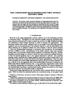
Fig. 1: The New Lucchi++ Mitochondria Benchmark Dataset. Left: Lucchi et al.’s original EPFL Hippocampus mitochondria segmentation benchmark dataset [18]. Right: Our neuroscientists re-annotate the original dataset to counter mitochondria boundary inconsistencies (examples in blue and red) and to correct misclassifications (yellow).

Megapixels/s) [26]. To counter the limited training data, we optimize our learning strategy by using significant data augmentation. We evaluate our method on Lucchi’s original EPFL Hippocampus dataset, the corrected Lucchi++ dataset, and the Kasthuri++ neocortex dataset. Our results confirm segmentation performance with a Jaccard index within the range of 0.845–0.90 and an average inference speed of 16 milliseconds which is suitable for real-time processing. We compare these numbers to previously published results and rank first among all real-time capable methods, and third overall. The created datasets and our mitochondria detection code are available as free and open source software3 .

2

Related Work

Early work on mitochondria detection is based on texture features or other traditional segmentation methods such as image filtering and connected components analysis [31, 7, 20]. All of these approaches do not consider shape and report rather low classification performance. Further research on hand-designed features for mitochondria detection improve accuracy only slightly, e.g. [28, 10, 30, 23]. 3

Code and data available at https://rhoana.org/mitochondria

4

Casser et al.

Segmentation performance closer to human annotators is first reported by Lucchi et al. [18]. The authors propose a graph partitioning scheme that operates on supervoxel output from a clustering algorithm. This paper also introduces the EPFL Hippocampus dataset with ground truth mitochondria labels – now a de facto benchmark in the community. Building upon their work, the same authors develop a general method for image segmentation by kernelizing features before applying a linear structured support vector machine [17]. Later, Lucchi presents a gradient descent based algorithm that further improves their detection performance [14]. Finally, the authors release two more papers advancing the field by explicitly modeling mitochondria membranes [15, 16]. Lucchi’s approach still yields the second best accuracy on the benchmark dataset. Recent work tends to avoid manual feature engineering altogether and instead relies on modern machine learning approaches. Several papers approach mitochondria detection using random forest classifiers but can not reach the performance reported by Lucchi [21, 27]. More promising are approaches based on convolutional neural networks (CNNs) which report excellent performance for biomedical segmentation tasks [24, 3, 25]. Oztel et al. propose a pixel-level mitochondria detector using a CNN and report very high performance on Lucchi’s benchmark dataset. Their technique allows for offline or batch processing after extensive refinement using their three step post-processing pipeline. Our method, while close, does not reach the performance of Oztel but allows for real-time processing with very low inference times. Our approach is most related to work by Cheng et al. who propose a similar CNN architecture [2]. However, the authors stress the need for a 3D U-Net approach [25], require non-standard factorized convolutions to reduce kernel dimensionality, and rely on advanced 3D data augmentation. We report slightly better performance on the benchmark dataset using our 2D classifier while offering the flexibility of processing single image slices. This is more robust to common errors such as missing slices and acquisition artifacts that often cause 3D alignment problems [5]. On a GPU, Cheng’s inference speed is not far from ours but requires computationally expensive 3D alignment and does not allow processing immediately after image acquisition.

3

Data

EPFL Hippocampus Data. This dataset was introduced by Lucchi et al. at the EPFL Computer Vision Laboratory and is publicly available4 [18]. The images were acquired using focused ion beam scanning electron microscopy (FIB-SEM) and taken from a 5 × 5 × 5µm section of the hippocampus of mouse brain, with the resolution of each voxel being approximately 5 × 5 × 5nm. The whole image stack is 2048 × 1536 × 1065vx and manually created mitochondria segmentation masks are available for two neighboring image stacks (each 1024 × 768 × 165vx). These two stacks are commonly used as separate training and testing data to 4

https://cvlab.epfl.ch/data/em

Fast Mitochondria Segmentation for Connectomics

5

Table 1: Expert Corrections of Mitochondria Datasets. We observed membrane inconsistencies and misclassifications in two publicly available datasets. We asked experts to correct these shortcomings in a consensus driven process and report the resulting changes. Experts spent 32-36 hours annotating each dataset. Kasthuri++

Lucchi++ before

after

# Mitochondria 99 80 avg. 2D area 2,761.69 3,319.36 avg. boundary distance 2.92 (±1.93) px

before

after

# Mitochondria 242 208 avg. 2D area 2,568.38 2,640.76 avg. boundary distance 0.6 (± 1.36) px

evaluate mitochondria detection algorithms [31, 7, 20, 27, 2, 22]. However, the community observed boundary inconsistencies in the provided ground truth annotations [2] and, indeed, our neuroscientists confirm that the labelings include misclassifications and inconsistently labeled membranes (Table 1). The Lucchi++ Dataset. Our experts re-annotated the two EPFL Hippocampus stacks. Our goal was to achieve consistency for all mitochondria membrane annotations and to correct any misclassifications in the ground truth labelings. First, a senior biologist manually corrected mitochondria membrane labelings using a publicly available in-house annotation software. For validation, two neuroscientists were then asked to separately proofread the labelings to judge membrane consistency. We then compared these judgments. In cases of disagreement between the neuroscientists, the biologist corrected the annotations until consensus between them was reached. The biologist annotated very precisely and only a handful of membranes had to be corrected after proofreading. To fix misclassifications, our biologist manually looked at every image slice of the two Hippocampus stacks for missing and wrongly labeled mitochondria. The resulting corrections were then again proofread by two neuroscientists until agreement was reached. In several cases it was only possible to identify structures as partial mitochondria by looking at previous sections in the image stacks. This could be the reason for misclassifications in the original Lucchi dataset (Figure 1). We summarize our corrections in Table 1. The Kasthuri++ Neocortex Dataset. We use the mitochondria annotations of the 3-cylinder mouse cortex volume of Kasthuri et al. [8]. The tissue is dense mammalian neuropil from layers 4 and 5 of the S1 primary somatosensory cortex, acquired using serial section electron microscopy (ssEM). Similar to Lucchi’s Hippocampus dataset, we noticed membrane inconsistencies within the mitochondria segmentation masks in this data. We asked our experts to correct these shortcomings through re-annotation of two neighboring sub-volumes leveraging the same process described above for the Lucchi++ dataset. The stack dimensions are 1463 × 1613 × 85vx and 1334 × 1553 × 75vx with a resolution of 3 × 3 × 30nm per voxel. Table 1 summarizes the corrections of these two stacks.

6

Casser et al.

Skip-Connections per Block

Skip-Connections per Block 2Mx2MxC

MxMxC

MxMxC

2Mx2MxC

2x Convolution +

Max. Pooling

512x512 3x3

2x Deconvolution +

Upsampling skip

2Mx2MxC 512x512

512 x 512 px

3x3

2x2

3x3

MxMxC

2Mx2MxC

512 x 512 px skip

2x2

MxMxC

3x3

2x2

3x3

2x2

skip

2xConv (Same)

Pooling

2xConv

(Max)

Dropout 0.2

Upsampling

Input

(Same)

skip

2xConv Output (Same)

Pooling (Max)

Dropout 0.2

Down-Block x4 Fig. 2: Our MitochondriaUp-Block Detector. Down-Block x4 x4 We extend a 2D U-Net architecture [25]

to output predictions at full resolution (512 × 512 pixels). Additionally, we are able to reduce the number of learnable parameters with less convolutional filters while maintaining high precision. To prevent overfitting due to limited training data, we employ extensive data augmentation.

4

Mitochondria Detection

Architecture. We build our mitochondria detector by adopting an architecture similar to the 2D U-Net architecture proposed by Ronneberger et al. [25]. The authors have reported excellent segmentation results on connectomics images similar to ours but target neurons rather than intracellular structures such as mitochondria. Our input and output sizes are 512 × 512 pixels, respectively, with the input being fed in as a grayscale image and the output being a binary mask, highlighting mitochondria as the positive class. We exclusively train and predict 2D image slices to allow processing immediately after image acquisition and to avoid waiting for a computationally expensive alignment procedure [5]. Differences to Original U-Net. Based on experimental evaluation, we are able to decrease the number of parameters compared to the original U-Net architecture. Specifically, we reduce the number of convolutional filters from 6,848 to 768 resulting in a significant reduction of learnable parameters from over 31 million to 1,958,533 without loss of classification accuracy. Unlike the original U-Net, we predict on full resolution meaning our input size equals our output size. This has the advantage that upsampling of predictions is not required, reducing computational overhead and increasing boundary precision. Data Augmentation. We employ an on-the-fly data augmentation pipeline, exploiting the specific nature of EM images as much as possible. We take images of any resolution as input. We then crop these images with dimensions of at least 512 pixels and randomly rotate them (bilinear interpolation). We also apply random bidirectional flipping. If needed, we down- or upsample the image before feeding it into the network to map from nanometers to pixels. Training and Inference. We minimize binary crossentropy loss using the Adam optimizer. Our network fully converges on average after training for about two hours on a modern Tesla GPU. We use a learning rate of 0.0005, a

2xConv

Upsampling

(Same)

Up-Block x4

Fast Mitochondria Segmentation for Connectomics

7

standard dropout of 0.2, and a batch size of 4. Our detector outputs accurate 2D-segmentation maps. For 3D reconstructions, however, we are able to include additional knowledge across sections as part of post-processing. Inspired by [22], we use a median filter along the z-dimension to filter mitochondria which are not present on consecutive sections (”Z-Filtering”).

5 5.1

Experiments Performance Metrics

In accordance with related work in this area, we mainly rely on Jaccard index and VOC score as segmentation performance metrics. Jaccard index, also known as Intersection over Union, can be calculated as J = T P +FT PP +F N where T P are the true positives, F P are the false positives of our positive class (foreground), and F N are false negatives (missing foreground). For a binary classification task like mitochondria detection, the VOC score is defined as the average of the Jaccard Index of the positive and negative class (foreground/background). We note that this score is not an accurate assessment of classifier performance since the background trivially adds to the score, and led to confusion in previous work [2]. However, in order to make our results more comparable, we report both measures. With inference times being crucial for this task, we also report both inference time and throughput of pixels per second.

(a) Image

(b) Results

(c) Luchi++ GT

(d) Error dist.

Fig. 3: Example results on EPFL Hippocampus. Our detector finds 16 out of 17 mitochondria (b) on the re-annotated Lucchi++ dataset with consistent mitochondria membrane annotation (c). The average spatial error distribution of the entire test stack confirms that errors are mainly found at the boundaries (d).

5.2

Experimental Setup

We evaluate our classifier on three datasets. All experiments involve training with the same, fixed parameters (Section 4) and predicting mitochondria on previously unseen test data. Optionally, we apply Z-filtering. We then threshold the predictions at 0.5 to generate binary masks that we use to compute similarity

8

Casser et al.

Table 2: Mitochondria Detection Results. We show the performance of our mitochondria detector in 2D and with Z-filtering on Lucchi’s original Hippocampus dataset, our re-annotated Lucchi++ dataset, and on the new Kasthuri++ dataset. We report testing accuracy, precision and recall including area-underthe-curve, the Jaccard index, and VOC-Score. Z-filtering is beneficial and does not require full 3D stack information. Accuracy Prec. / Recall (AUC) Jaccard VOC EPFL Hippocampus 2D U-Net with Z-filtering

0.993 0.994

0.932 / 0.939 (0.982) 0.946 / 0.937 (0.986)

0.878 0.935 0.890 0.942

Lucchi++ 2D U-Net with Z-filtering

0.992 0.993

0.963 / 0.919 (0.986) 0.974 / 0.922 (0.992)

0.888 0.940 0.900 0.946

Kasthuri++ 2D U-Net with Z-filtering

0.995 0.995

0.925 / 0.908 (0.969) 0.932 / 0.902 (0.971)

0.845 0.920 0.846 0.920

measures with respect to the manual ground truth labels. We also compute average prediction times of multiple runs to determine inference speed. Evaluation on the EPFL Hippocampus Dataset. Lucchi’s dataset is the de facto benchmark in the community despite known shortcomings. Evaluating on this dataset allows us to compare against existing mitochondria detection methods. However, some of these methods report VOC score as the Jaccard index which led to confusion and was previously noticed by the community [2]. Unfortunately, it is not possible to recalculate their individual results because either code, pre-computed features, or parameters are not available. However, whenever the Jaccard index is missing, we infer lower bounds by using other reported scores and enable fair comparisons. Evaluation on Lucchi++. We detect mitochondria on the new version of the EPFL Hippocampus dataset with consistent boundaries. Evaluation on Kasthuri++. In contrast to Lucchi’s data, the Kasthuri++ dataset is from the neocortex using a serial section electron microscope. Additionally, the resolution of this dataset is nearly twice as high. This dataset allows us to see if our mitochondria detector generalizes well to diverse data samples.

6

Results

Detection Accuracy and Ability to Generalize. Table 2 summarizes our mitochondria detection performance on previously unseen test stacks of the EPFL Hippocampus dataset, our re-annotated Lucchi++ dataset, and the new

Fast Mitochondria Segmentation for Connectomics

9

Table 3: Performance Comparison on EPFL Hippocampus. We compare our method to previously published approaches. We report performance as Jaccard and VOC scores, ordered by Jaccard (the higher, the better). If not reported in the respective papers, we infer lower bounds from other scores as indicated by +. Methods inherently requiring pre-alignment are marked as (†). Method

Description

Jaccard VOC Real-Time

Oztel 2017 [22] Lucchi 2015 [16] Ours Cheng 2017 [2] Ours Ours Cheng 2017 [2] Cetina 2018 [1] Marquez 2014 [19] Lucchi 2014 [15] Lucchi 2013 [14] Lucchi 2012 [17] Lucchi 2011 [18]

Sliding window CNN + post-proc. Working set + inference autostep With Z-filtering 3D U-Net (†) Human Expert 2D U-Net 2D U-Net PIBoost (multi-class boosting) Random fields Ccues + 3-class CRF Working set + inference k. Kernelized SSVM / CRF Learned f.

0.907 0.895+ 0.890 0.889 0.884 0.878 0.865 0.76 0.762 0.741 0.734+ 0.680+ 0.600+

0.948 0.942 0.942 0.938 0.935 0.928 0.867 0.840 0.800

3 3 3 3

Kasthuri++ dataset. Averaged across all datasets, we measure a Jaccard score of 0.870 (±0.018) in 2D, and 0.879 (±0.023) with Z-filtering using depth d ∼ 15. Our average Precision and Recall AUC is 0.979 (±0.007) and average testing accuracy is greater than 0.993 (±0.001). The combination of these measures reflect very high mitochondria detection performance with little variance and shows that our method generalizes well to diverse data (Kasthuri++). Inference in Real-time. We measure mitochondria segmentation times in Table 4. The average throughput of our method, depending on the dataset’s structure, is between 11 and 35.4 Megapixels/s which consistently keeps up or outperforms the acquisition time of modern single beam electron microscopes (11 Megapixels/s) [26]. We are able to process a 512 × 512 pixels region on average in 16 milliseconds, allowing mitochondria detection in real-time using a modern Titan GPU. We also measure inference using Lucchi et al.’s method [16] on the EPFL Hippocampus dataset with a modern CPU (12x 3.4 GHz Intel Core i7 - since it is not executable on GPU). Their method is significantly slower, and with a throughput of about 0.16 Megapixels/s far from real-time capable. Comparison with Other Methods and Human Performance. We list previously published results on the EPFL Hippocampus dataset in Table 3 and order them by classification performance (high to low). Our detector yields the highest Jaccard score of all real-time methods. While the difference in accuracy to Chengs’ 3D U-Net [2] is only marginal, we predict single images, require no pre-alignment and thus, even with Z-filtering as post-processing, require less

10

Casser et al.

Table 4: Inference in Real-time. We measure the time required to predict the testing stacks, using a batchsize of 1. Our method is able to predict faster than the acquisition speed of modern electron microscopes (11 MP/s) and thus enables real-time inference. For the EPFL Hippocampus dataset we also report inference time of Lucchi et al. [16] which ranks second in overall segmentation accuracy. GPU Full stack [s]

Slice (512 × 512px) [s] Throughput [MP/s]

EPFL Hippocampus Lucchi et al. [16] Ours (2D U-Net) Ours (with Z-filtering)

3 3

815.2 (±41) 0.609 (±0.02700) 8.570 (±0.072) 0.016 (±0.00004) 11.659 (±0.0082) 0.023 (±0.00002)

0.16 (±0.007) 15.142 (±0.126) 11.130 (±0.008)

Lucchi++ Ours (2D U-Net) Ours (with Z-filtering)

3 3

8.644 (±0.202) 0.016 (±0.00009) 11.785 (±0.0141) 0.022 (±0.00003)

15.019 (±0.334) 11.010 (±0.013)

Kasthuri++ Ours (2D U-Net) Ours (with Z-filtering)

3 3

4.387 (±0.0317) 0.016 (±0.00006) 5.122 (±0.0092) 0.017 (±0.00001)

35.421 (±0.255) 30.332 (±0.054)

computation for end-to-end processing. Compared to offline methods, we rank third with a Jaccard difference of 0.017. We also compare performance to expert annotators on the original EPFL Hippocampus dataset in Table 3. Cheng’s 3D U-Net [2] and our 2D U-Net with Z-filtering yield better Jaccard scores than human annotators (a difference of 0.005 and 0.006, respectively). This is not surprising since CNN architectures are recently able to outperform humans on connectomics segmentation tasks [11].

7

Conclusions

The segmentation of mitochondria during the image acquisition process is possible. Our end-to-end detector uses 2D images and automatically produces accurate segmentation masks of high quality in real-time. This is crucial as connectomics datasets approach petabytes in size. By predicting mitochondria in 2D, parallelization is as trivial as processing sections individually which can further increase throughput. We also confirm previously reported inconsistencies in publicly available segmentation datasets of mitochondria and fix the shortcomings in two available ground truth annotations. We provide the datasets and our code as free and open source in order to facilitate further research. For instance, 2D mitochondria detection could generate features to improve robustness and speed of current EM image alignment procedures.

REFERENCES

11

References [1] Kendrick Cetina, Jos´e M Buenaposada, and Luis Baumela. “Multi-class segmentation of neuronal structures in electron microscopy images”. In: BMC bioinformatics 19.1 (2018), p. 298. [2] Hsueh-Chien Cheng and Amitabh Varshney. “Volume segmentation using convolutional neural networks with limited training data”. In: Image Processing (ICIP), IEEE International Conference on. 2017, pp. 590–594. [3] Dan Ciresan et al. “Deep neural networks segment neuronal membranes in electron microscopy images”. In: Advances in Neural Information Processing Systems. 2012, pp. 2843–2851. [4] James E Darnell, Harvey Lodish, David Baltimore, et al. Molecular cell biology. Vol. 2. Scientific American Books New York, 1990. [5] Daniel Haehn et al. “Scalable Interactive Visualization for Connectomics”. In: Informatics. Vol. 4. 3. MDPI. 2017, p. 29. [6] Moritz Helmst¨adter, Kevin L Briggman, and Winfried Denk. “High-accuracy neurite reconstruction for high-throughput neuroanatomy.” In: Nature Neuroscience 14.8 (2011), pp. 1081–1088. [7] Sylvain Jaume et al. “A Multiscale Parallel Computing Architecture for Automated Segmentation of the Brain Connectome”. In: IEEE Transactions on Biomedical Engineering 59.1 (2012), pp. 35–38. [8] Narayanan Kasthuri et al. “Saturated Reconstruction of a Volume of Neocortex”. In: Cell 162.3 (2015), pp. 648–661. [9] Verena Kaynig et al. “Large-scale automatic reconstruction of neuronal processes from electron microscopy images”. In: Medical Image Analysis 22.1 (2015), pp. 77–88. [10] Ritwik Kumar, Amelio V´azquez-Reina, and Hanspeter Pfister. “Radon-Like Features and their Application to Connectomics”. In: Computer Vision and Pattern Recognition Workshops (CVPRW). IEEE. 2010, pp. 186–193. [11] Kisuk Lee et al. “Superhuman accuracy on the SNEMI3D connectomics challenge”. In: arXiv preprint arXiv:1706.00120 (2017). [12] Jeff W. Lichtman and W. Denk. “The Big and the Small: Challenges of Imaging the Brain’s Circuits”. In: Science 334.6056 (2011), pp. 618–623. [13] Jeff W. Lichtman, Hanspeter Pfister, and Nir Shavit. “The big data challenges of connectomics”. In: Nat Neurosci 17.11 (Nov. 2014). Perspective, pp. 1448–1454. issn: 1097-6256. [14] Aur´elien Lucchi, Yunpeng Li, and Pascal Fua. “Learning for Structured Prediction using Approximate Subgradient Descent with Working Sets”. In: Computer Vision and Pattern Recognition (CVPR). 2013, pp. 1987–1994. [15] Aur´elien Lucchi et al. “Exploiting Enclosing Membranes and Contextual Cues for Mitochondria Segmentation”. In: International Conference on Medical Image Computing and Computer-Assisted Intervention. Springer. 2014, pp. 65–72. [16] Aur´elien Lucchi et al. “Learning Structured Models for Segmentation of 2-D and 3-D Imagery”. In: IEEE Transactions on Medical Imaging 34.5 (2015), pp. 1096–1110.

12

REFERENCES

[17] Aur´elien Lucchi et al. “Structured Image Segmentation using Kernelized Features”. In: Computer Vision–ECCV 2012. Springer, 2012, pp. 400–413. [18] Aur´elien Lucchi et al. “Supervoxel-Based Segmentation of Mitochondria in EM Image Stacks with Learned Shape Features”. In: IEEE Transactions on Medical Imaging 31.2 (2012), pp. 474–486. [19] Pablo M´arquez-Neila et al. “Non-parametric higher-order random fields for image segmentation”. In: European Conference on Computer Vision. Springer. 2014, pp. 269–284. [20] Rajesh Narasimha et al. “Automatic Joint Classification and Segmentation of Whole Cell 3D Images”. In: Pattern Recognition 42.6 (2009). [21] Juan Nunez-Iglesias et al. “Graph-based Active Learning of Agglomeration (GALA): A Python library to segment 2D and 3D neuroimages”. In: Frontiers in Neuroinformatics 8.34 (2014). issn: 1662-5196. [22] Ismail Oztel et al. “Mitochondria segmentation in electron microscopy volumes using deep convolutional neural network”. In: International Conference on Bioinformatics and Biomedicine (BIBM). 2017, pp. 1195–1200. [23] Alex J. Perez et al. “A Workflow for the Automatic Segmentation of Organelles in Electron Microscopy Image Stacks”. In: Frontiers in neuroanatomy 8 (2014), p. 126. [24] Tran Minh Quan, David GC Hilderbrand, and Won-Ki Jeong. “FusionNet: A deep fully residual convolutional neural network for image segmentation in connectomics”. In: arXiv preprint arXiv:1612.05360 (2016). [25] Olaf Ronneberger, Philipp Fischer, and Thomas Brox. “U-Net: Convolutional Networks for Biomedical Image Segmentation”. In: International Conference on Medical Image Computing and Computer Assisted Intervention. Springer. 2015, pp. 234–241. [26] Richard Schalek et al. “Imaging a 1 mm 3 Volume of Rat Cortex Using a MultiBeam SEM”. In: Microscopy and Microanalysis 22.S3 (2016). [27] Mojtaba Seyedhosseini, Mark H Ellisman, and Tolga Tasdizen. “Segmentation of Mitochondria in Electron Microscopy Images using Algebraic Curves”. In: Biomedical Imaging (ISBI), 2013 IEEE 10th International Symposium on. IEEE. 2013, pp. 860–863. [28] Kevin Smith, Alan Carleton, and Vincent Lepetit. “Fast Ray Features for Learning Irregular Shapes”. In: Computer Vision, 2009 IEEE 12th International Conference on. IEEE. 2009, pp. 397–404. [29] Adi Suissa-Peleg et al. “Automatic Neural Reconstruction from Petavoxel of Electron Microscopy Data”. In: Microscopy and Microanalysis 22.S3 (2016), pp. 536–537. [30] Amelio Vazquez-Reina et al. “Segmentation Fusion for Connectomics”. In: International Conference on Computer Vision (ICCV). IEEE. 2011. [31] Shiv Vitaladevuni et al. “Mitochondria detection in electron microscopy images”. In: Workshop on Microscopic Image Analysis with Applications in Biology. Vol. 42. 2008. [32] Massimo Zeviani and Stefano Di Donato. “Mitochondrial disorders”. In: Brain 127.10 (2004), pp. 2153–2172.