Fast Neighborhood Graph Search using Cartesian Concatenation
arXiv:1312.3062v1 [cs.CV] 11 Dec 2013
Jingdong Wang Jing Wang Gang Zeng Rui Gan Shipeng Li Baining Guo
Abstract In this paper, we propose a new data structure for approximate nearest neighbor search. This structure augments the neighborhood graph with a bridge graph. We propose to exploit Cartesian concatenation to produce a large set of vectors, called bridge vectors, from several small sets of subvectors. Each bridge vector is connected with a few reference vectors near to it, forming a bridge graph. Our approach finds nearest neighbors by simultaneously traversing the neighborhood graph and the bridge graph in the best-first strategy. The success of our approach stems from two factors: the exact nearest neighbor search over a large number of bridge vectors can be done quickly, and the reference vectors connected to a bridge (reference) vector near the query are also likely to be near the query. Experimental results on searching over large scale datasets (SIFT, GIST and HOG) show that our approach outperforms state-of-the-art ANN search algorithms in terms of efficiency and accuracy. The combination of our approach with the IVFADC system [20] also shows superior performance over the BIGANN dataset of 1 billion SIFT features compared with the best previously published result.
Jingdong Wang Microsoft Research e-mail:
[email protected] Jing Wang, Peking University e-mail:
[email protected] Gang Zeng, Peking University e-mail:
[email protected] Rui Gan Peking University e-mail:
[email protected] Shipeng Li Microsoft Research e-mail:
[email protected] Baining Guo Microsoft Research e-mail:
[email protected]
1
2
Jingdong Wang Jing Wang Gang Zeng Rui Gan Shipeng Li Baining Guo
1 Introduction Nearest neighbor (NN) search is a fundamental problem in machine learning, information retrieval and computational geometry. It is also a crucial step in many vision and graphics problems, such as shape matching [13], object retrieval [31], feature matching [8, 37], texture synthesis [25], image completion [16] and so on. Recently, the nearest neighbor search problem attracts more attentions in computer vision because of the popularity of large scale and high-dimensional multimedia data. The simplest solution to NN search is linear scan, comparing each reference vector to the query vector. The search complexity is linear with respect to both the number of reference vectors and the data dimensionality. Apparently, it is too timeconsuming and does not scale well in large scale and high-dimensional problems. Algorithms, including the KD tree [3, 5, 6, 12], BD trees [3], cover tree [7], nonlinear embedding [18] and so on, have been proposed to improve the search efficiency. However, for high-dimensional cases it turns out that such approaches are not much more efficient than linear scan and cannot satisfy the practical requirement. Therefore, a lot of efforts have been turned to approximate nearest neighbor (ANN) search, such as KD trees with its variants, hashing algorithms, neighborhood graph search, and inverted indices. In this paper, we propose a new data structure for approximate nearest neighbor search 1 . This structure augments the neighborhood graph with a bridge graph that is able to boost approximate nearest neighbor search performance. Inspired by the product quantization technology [4, 20], we adopt Cartesian concatenation (or Cartesian product), to generate a large set of vectors, which we call bridge vectors, from several small sets of subvectors to approximate the reference vectors. Each bridge vector is then connected to a few reference vectors that are near enough to it, forming a bridge graph. Combining the bridge graph with the neighborhood graph built over reference data vectors yields an augmented neighborhood graph. The ANN search procedure starts by finding the nearest bridge vector to the query vector, and discovers the first set of reference vectors connected to such a bridge vector. Then the search simultaneously traverses the bridge graph and the neighborhood graph in the best-first manner using a shared priority queue. The advantages of adopting the bridge graph lie in two-fold. First, computing the distances from bridge vectors to the query is very efficient, for instance, the computation for 1000000 bridge vectors that are formed by 3 sets of 100 subvectors takes almost the same time as that for 100 vectors. Second, the best bridge vector is most likely to be very close to true NNs, allowing the ANN search to quickly reach true NNs through bridge vectors. We evaluate the proposed approach by the feature matching performance on SIFT and HOG features, and the performance of searching similar images over tiny images [38] with GIST features. We show that our approach achieves significant improvements compared with the state-of-the-art in terms of accuracy and search 1
A conference version appeared in [45].
Fast Neighborhood Graph Search using Cartesian Concatenation
3
time. We also demonstrate that our approach in combination with the IVFADC system [20] outperforms the state-of-the-art over the BIGANN dataset of 1 billion SIFT vectors [21].
2 Literature review Nearest neighbor search in the d-dimensional metric space Rd is defined as follows: given a query q, the goal is to find an element NN(q) from the database X = {x1 , · · · , xn } so that NN(q) = arg minx∈X dist(q, x). In this paper, we assume that Rd is an Euclidean space and dist(q, x) = kq − xk2, which is appropriate for most problems in multimedia search and computer vision. There are two types of ANN search problems. One is error-constrained ANN search that terminates the search when the minimum distance found up to now lies in some scope around the true minimum (or desired) distance. The other one is timeconstrained ANN search that terminates the search when the search reaches some prefixed time (or equivalently examines a fixed number of data points). The latter category is shown to be more practical and give better performance. Our proposed approach belongs to the latter category. The ANN search algorithms can be roughly divided into four categories: partition trees, neighborhood graph, compact codes (hashing and source coding), and inverted index. The following presents a short review of the four categories.
2.1 Partition trees The partition tree based approaches recursively split the space into subspaces, and organize the subspaces via a tree structure. Most approaches select hyperplanes or hyperspheres according to the distribution of data points to divide the space, and accordingly data points are partitioned into subsets. The KD trees [6, 12], using axis-aligned hyperplane to partition the space, have been modified to find ANNs. Other trees using different partition schemes, such as BD tress [3], metric trees [9, 26, 28, 51], hierarchical k-means tree [30], and randomized KD trees [22, 35, 47], have been proposed. FLANN [29] aims to find the best configuration of the hierarchical k-means trees and randomized KD trees, and has been shown to work well in practice. In the query stage, the branch-and-bound methodology [6] is usually adopted to search (approximate) nearest neighbors. This scheme needs to traverse the tree in the depth-first manner from the root to a leaf by evaluating the query at each internal node, and pruning some subtrees according to the evaluation and the currently-found nearest neighbors. The current state-of-the-art search strategy, priority search [3] or best-first [5], maintains a priority queue to access subtrees in order so that the data points with large probabilities being true nearest neighbors are first accessed. It has
4
Jingdong Wang Jing Wang Gang Zeng Rui Gan Shipeng Li Baining Guo
been shown that best-first search (priority search) achieves the best performance for ANN search, while the performance might be worse for Exact NN search than the algorithms without using best-first search.
2.2 Neighborhood graph search The data structure of the neighborhood graph is a directed graph connecting each vector and its nearest neighbors. Usually a R-NN graph, that connects each vector to its R nearest neighbors, is used. Various algorithms based on neighborhood graph [1, 2, 5, 15, 33, 34, 41] are developed for ANN search has been. The basic procedure of neighborhood graph search starts from one or several seeding vectors, and puts them into a priority queue with the distance to the query being the key. Then the process proceeds by popping the top one in the queue, i.e., the nearest one to the query, and expanding its neighborhood vectors (from neighborhood graph), among which the vectors that have not been visited are pushed into the priority queue. This process iterates till a fixed number of vectors are accessed. Using neighborhood vectors of a vector as candidates has two advantages. One is that extracting the candidates is very cheap and only takes O(1) time. The other is that if one vector is close to the query, its neighborhood vectors are also likely to be close to the query. The main research efforts consists of two aspects. One is to build an effective neighborhood graph [1, 33]. The other is to design efficient and effective ways to guide the search in the neighborhood graph, including presetting the seeds created via clustering [33, 34], picking the candidates from KD tress [2], iteratively searching between KD trees and the neighborhood graph [41]. In this paper, we present a more effective way, combining the neighborhood graph with a bridge graph, to search for approximate nearest neighbors.
2.3 Compact codes The compact code approaches transform each data vector into a small code, using the hashing or source coding techniques. Usually the small code takes much less storage than the original vector, and particularly the distance in the small code space, e.g., hamming distance or using lookup table can be much more efficiently evaluated than in the original space. Locality sensitive hashing (LSH) [10], originally used in a manner similar to inverted index, has been shown to achieve good theory guarantee in finding near neighbors with probability, but it is reported not as good as KD trees in practice [29]. Multi-probe LSH [27] adopts the search algorithm similar to priority search, achieving a significant improvement. Nowadays, the popular usage of hashing is to use the hamming distance between hash codes to approximate the distance in the original space and then adopt linear scan to conduct the search. To make the best of the
Fast Neighborhood Graph Search using Cartesian Concatenation
5
data, recently, various data-dependent hashing algorithms are proposed by learning hash functions using metric learning-like techniques, including optimized kernel hashing [17], learned metrics [19], learnt binary reconstruction [23], kernelized LSH [24], and shift kernel hashing [32], semi-supervised hashing [40], (multidimensional) spectral hashing [48, 49], spectral hashing [49], iterative quantization [14], complementary hashing [50] and order preserving hashing [44]. The source coding approach, product quantization [20], divides the vector into several (e.g., M) bands, and quantizes reference vectors for each band separately. Then each reference vector is approximated by the nearest center in each band, and the index for the center is used to represent the reference vector. Accordingly, the distance in the original space is approximated by the distance over the assigned centers in all bands, which can be quickly computed using precomputed lookup tables storing the distances between the quantization centers of each band separately.
2.4 Inverted index Inverted index is composed of a set of inverted lists each of which contains a subset of the reference vectors. The query stage selects a small number of inverted lists, regards the vectors contained in the selected inverted lists as the NN candidates, and rerank the candidates, using the distance computed from the original vector or using the distance computed from the small codes followed by a second-reranking step using the distance computed from the original vector, to find the best candidates. The inverted index algorithms are widely used for very large datasets of vectors (hundreds of million to billions) due to its small memory cost. Such algorithms usually load the inverted index (and possibly extra codes) into the memory and store the raw features in the disk. A typical inverted index is built by clustering algorithms, e.g., [4, 20, 30, 36, 42], and is composed of a set of inverted lists, each of which corresponds to a cluster of reference vectors. Other inverted indices include hash tables [10], tree codebooks [6] and complementary tree codebooks [39].
3 Preliminaries This section gives short introductions on several algorithms our approach depends on: neighborhood graph search, product quantization, and the multi-sequence search algorithm.
6
Jingdong Wang Jing Wang Gang Zeng Rui Gan Shipeng Li Baining Guo
3.1 Neighborhood graph search A neighborhood graph of a set of vectors X = {x1 , · · · , xn } is a directed graph that organizes data vectors by connecting each data point with its neighboring vectors. The neighborhood graph is denoted as G = {(vi , Ad j[vi ])}ni=1 , where vi corresponds to a vector xi and Ad j[vi ] is a list of nodes that correspond to its neighbors. The ANN search algorithm proposed in [2], we call local neighborhood graph search, is a procedure that starts from a set of seeding points as initial NN candidates and propagates the search by continuously accessing their neighbors from previously-discovered NN candidates to discover more NN candidates. The bestfirst strategy [2] is usually adopted for local neighborhood expansion2. To this end, a priority queue is used to maintain the previously-discovered NN candidates whose neighborhoods are not expanded yet, and initially contains only seeds. The best candidate in the priority queue is extracted out, and the points in its neighborhood are discovered as new NN candidates and then pushed into the priority queue. The resulting search path, discovering NN candidates, may not be monotone, but always attempts to move closer to the query point without repeating points. As a local search that finds better solutions only from the neighborhood of the current solution, the local neighborhood graph search will be stuck at a locally optimal point and has to conduct exhaustive neighborhood expansions to find better solutions. Both the proposed approach and the iterated approach [41] aim efficiently find solutions beyond local optima.
3.2 Product quantization The idea of product quantization is to decomposes the space into a Cartesian product of M low dimensional subspaces and to quantize each subspace separately. A vector x is then decomposed into M subvectors, x1 , · · · , xM , such that xT = [(x1 )T (x2 )T · · · (xM )T ]. Let the quantization dictionaries over the M subspaces be C1 , C2 , · · · , CM with Cm being a set of centers {cm1 , · · · , cmK }. A vector x is represented by a short code composed of its subspace quantization indices, {k1 , k2 , · · · , kM }. Equivalently, (1) C(1) 0 · · · 0 b 0 C(2) · · · 0 b(2) x= . .. .. .. .. , .. . . . . (M) (M) 0 0 ··· C b
(1)
where b(m) is a vector in which the km entry is 1 and all others are 0. 2 The depth-first search strategy can also be used. Our experiments show that the performance is much worse than the best-first search.
Fast Neighborhood Graph Search using Cartesian Concatenation
7
Given a query q, the asymmetric scheme divides q into M subvectors q1 , qM , and computes M distance arrays {d1 , · · · , dM } (for computation efficiency, store the square of the Euclidean distance) with the centers of the M subspaces. For a database point encoded as {k1 , k2 , · · · , kM }, the square of the Euclidean distance is approximated as ∑M m=1 dmkm , which is called asymmetric distance. The application of product quantization in our approach is different from applications to fast distance computation [20] and code book construction [4], the goal of Cartesian product in this paper is to build a bridge to connect the query and the reference vectors through bridge vectors.
3.3 Multi-sequence search Given several monotonically increasing sequences, {Sb }Bb=1 where Si is a sequence, sb (1), sb (2), . . . , sb (Lb ), with sb (l) < sb (l + 1), the multi-sequence search algorithm [4] is able to efficiently traverse the set of B-tuples {(s1 (i1 ), s2 (i2 ), . . . , sB (iB ))|ib = 1 . . . Lb } in order of increasing the sum s1 (i1 ) + s2 (i2 ) + · · · + sB (iB ). The algorithm uses a min-priority queue of the tuples (i1 , i2 , . . . , iB ) with the key being the sum s1 (i1 ) + s2 (i2 ) + · · · + sB (iB ). It starts by initializing the queue with a tuple (1, 1, . . . , 1). At step t, the tuple with top priority (the minimum sum), (t) (t) (t) (i1 , i2 , . . . , iB ), is popped from the queue and regarded as the tth best tuple whose sum is the tth smallest. At the same time, the tuple (i1 , i2 , . . . , iB ), if all its preceding tuples, {(i′1 , i′2 , . . . , i′B )|i′b = ib , ib − 1} − {(i1 , i2 , . . . , iB )} have already been pushed into the queue is pushed into the queue. As a result, the multi-sequence algorithm produces a sequence of B-tuples in order of increasing the sum and can stop at step t − 1 if the best t B-tuples are required. It is shown in [4] that the time cost of extracting the best t B-tuples is t logt.
4 Approach The database X contains N d-dimensional reference vectors, X = {x1 , x2 , · · · , xN }, xi ∈ Rd . Our goal is to build an index structure using the bridge graph such that, given a query vector q, its nearest neighbors can be quickly discovered. In this section, we first describe the index structure and then show the search algorithm.
4.1 Data structure Our index structure consists of two components: a bridge graph that connects bridge vectors and their nearest reference vectors, and a neighborhood graph that connects each reference vector to its nearest reference vectors.
8
Jingdong Wang Jing Wang Gang Zeng Rui Gan Shipeng Li Baining Guo
Bridge vectors. Cartesian concatenation is an operation that builds a new set out of a number of given sets. Given m sets, {S1 , S2 , · · · , Sm }, where each set, in our case, contains a set of di -dimensional subvectors such that ∑m i=1 di = d, the Cartesian concatenation of those sets is defined as follows, T T T T Y = ×m i=1 Si , {y j = [y j1 y j2 · · · y jm ] |y ji ∈ Si }.
Here y j is a d-dimensional vector, and there exist ∏m i=1 ni vectors (ni = |Si | is the number of elements in Si ) in the Cartesian concatenation Y . Without loss of generality, we assume that n1 = n2 = · · · = nm = n for convenience. There is a nice property that identifying the nearest one from Y to a query only takes O(dn) time rather than O(dnm ), despite that the number of elements in Y is nm . Inspired by this property, we use the Cartesian concatenation Y , called bridge vectors, as bridges to connect the query vector with the reference vectors. Computing bridge vectors. We propose to use product quantization [20], which aims to minimize the distance of each vector to the nearest concatenated center derived from subquantizers, to compute bridge vectors. This ensures that the reference vectors discovered through one bridge vector are not far away from the query and hence the probability that those reference vectors are true NNs is high. It is also expected that the number of reference vectors that are close enough to at least one bridge vector should be as large as possible (to make sure that enough good reference vectors can be discovered merely through bridge vectors) and that the average number of the reference vectors discovered through each bridge vector should be small (to make sure that the time cost to access them is low). To this end, we generate a large amount of bridge vectors. Such a requirement is similar to [20] for source coding and different from [4] for inverted indices. Augmented neighborhood graph. The augmented neighborhood graph is a combination of the neighborhood graph G¯ over the reference database X and the bridge graph B between the bridge vectors Y and the reference vectors X . The neighborhood graph G¯ is a directed graph. Each node corresponds to a point xi , and is also denoted as xi for convenience. Each node xi is connected with a list of nodes that correspond to its neighbors, denoted byAd j[xi ]. The bridge graph B is constructed by connecting each bridge vector y j in Y to its nearest vectors Ad j[yi ] in X . To avoid expensive computation cost, we build the bridge graph approximately by finding top t (typically 100 in our experiments) nearest bridge vectors for each reference vector and then keeping top b nearest (typically 5 in our experiments) reference vectors for each bridge vector, which is efficient and takes O(Nt(logt + b)) time. The bridge graph is different from the inverted multi-index [4]. In the inverted multi-index, each bridge vector y contains a list of vectors that are closer to y than all other bridge vectors, while in our approach each bridge is associated with a list of vectors that are closer to y than all other reference data points.
Fast Neighborhood Graph Search using Cartesian Concatenation
9
10
10
6
6
6 7
1
7
2 4
4
9
9
8
8
12
8 5 11
Y
X
X
(a) Iteration 1
Y
X
X
(b) Iteration 2
Y
X
X
(c) Iteration 3
Y
X
X
(d) Iteration 4
Fig. 1 An example illustrating the search process. Y → X : the bridge graph, and X → X : the neighborhood graph. The white numbers are the distances to the query. Magenta denotes the vectors in the main queue, green represents the vector being popped out from the main queue, and black indicates the vectors whose neighborhoods have already been expanded
4.2 Query the augmented neighborhood graph To make the description clear, without loss of generality, we assume there are two sets of n subvectors, S1 = {y11 , y12 , · · · , y1n } and S2 = {y21 , y22 , · · · , y2n }. Given a query q consisting of two subvectors q1 and q2 , the goal is to generate a list of T (T ≪ N) candidate reference points from X where the true NNs of q are most likely to lie. This is achieved by traversing the augmented neighborhood graph in a best-first strategy. We give a brief overview of the ANN search procedure over a neighborhood graph before describing how to make use of bridge vectors. The algorithm begins with a set of (one or several) vectors Ps = {p} that are contained in the neighborhood graph. It maintains a set of nearest neighbor candidates (whose neighborhoods have not been expanded), using a min-priority queue, which we call the main queue, with the distance to the query as the key. The main queue initially contains the vectors in Ps . The algorithm proceeds by iteratively expanding the neighborhoods in a best-first strategy. At each step, the vector p∗ with top priority (the nearest one to q) is popped from the queue. Then each neighborhood vector in Ad j[p∗ ] is inserted to the queue if it is not visited, and at the same time it is added to the result set (maintained by a max-priority queue with a fixed length depending on how many nearest neighbors are expected). To exploit the bridge vectors, we present an extraction-on-demand strategy, instead of fetching all the bridge vectors to the main queue, which leads to expensive cost in sorting them and maintaining the main queue. Our strategy is to maintain the main queue such that it consists of only one bridge vector if available. To be specific, if the top vector p∗ in the main queue is a reference vector, the algorithm proceeds as usual, the same to the above procedure without using bridge vectors. If the top vector is a bridge vector, we first insert its neighbors Ad j[p∗ ] into the main queue and the result set, and in addition we find the next nearest bridge vector (to the
10
Jingdong Wang Jing Wang Gang Zeng Rui Gan Shipeng Li Baining Guo
query q) and insert it to the main queue. The pseudo code of the search algorithm is given in Algorithm 1 and an example process is illustrated in Figure 1. Before traversing the augmented neighborhood graph, we first process the bridge vectors, and compute the distances (the square of the Euclidean distance) from q1 to the subvectors in S1 and from q2 to the subvectors in S2 , and then sort the subvectors in the order of increasing distances, respectively. We denote the sorted subvectors as {y1i1 , · · · , y1in } and {y2j1 , · · · , y2jn }. As the size n of S1 and S2 is typically not large (e.g., 100 in our case), the computation cost is very small (See details in Section 6). The extraction-on-demand strategy needs to visit the bridge vector one by one in the order of increasing distance from q. It is easily shown that dist2 (q, y) = dist2 (q1 , y1 ) + dist2 (q2 , y2 ), where y is consists of y1 and y2 . Naturally, yi1 , j1 , composed of y1i1 and y2i1 , is the nearest one to q. The multi-sequence algorithm (corresponding to ExtractNextNearestBridgeVector() in Algorithm 1) is able to fast produce a sequence of pairs (ik , jl ) so that the corresponding bridge vectors are visited in the order of increasing distances to the query q. The algorithm is very efficient and producing the t-th bridge vector only takes O(log(t)) time. Slightly different from extracting a fixed number of nearest bridge vectors once [4], our algorithm automatically determines when to extract the next one, that is when there is no bridge vector in the main queue.
5 Experiments 5.1 Setup We perform our experiments on three large datasets: the first one with local SIFT features, the second one with global GIST features, and the third one with HOG features, and a very large dataset, the BIGANN dataset of 1 billion SIFT features [21]. The SIFT features are collected from the Caltech 101 dataset [11]. We extract maximally stable extremal regions (MSERs) for each image, and compute a 128dimensional byte-valued SIFT feature for each MSER. We randomly sample 1000K SIFT features and 100K SIFT features, respectively as the reference and query set. The GIST features are extracted on the tiny image set [38]. The GIST descriptor is a 384-dimensional byte-valued vector. We sample 1000K images as the reference set and 100K images as the queries. The HOG descriptors are extracted from Flickr images, and each HOG descriptor is a 512-dimensional byte-valued vector. We sample 10M HOG descriptors as the reference set and 100K as the queries. The BIGANN dataset [21] consists of 1B 128-dimensional byte-valued vectors as the reference set and 10K vectors as the queries. We use the accuracy score to evaluate the search quality. For k-ANN search, the accuracy is computed as r/k, where r is the number of retrieved vectors that are contained in the true k nearest neighbors. The true nearest neighbors are computed
Fast Neighborhood Graph Search using Cartesian Concatenation
11
Algorithm 1 ANN search over the augmented neighborhood graph /* q: the query; X : the reference data vectors; Y : the set of bridge vectors; G: the augmented neighborhood graph; Q: the main queue; R: the result set; T : the maximum number of discovered vectors; */ Procedure ANNSearch(q, X , Y , G, Q, R, T ) 1. /* Mark each reference vector undiscovered */ 2. for each x ∈ X do 3. Color[x] ← white; 4. end for 5. /* Extract the nearest bridge vector */ 6. (y, D) ← ExtractNextNearestBridgeVector(Y ); 7. Q ← (y, D); 8. t ← 0 9. /* Start the search */ 10. while (Q 6= 0/ && t 6 T ) do 11. /* Pop out the best candidate vector and expand its neighbors */ 12. (p, D) ← Q. pop(); 13. for each x ∈ Ad j[p] do 14. if Color[x] = white then 15. D ← dist(q, x); 16. Q ← (x, D); 17. Color[x] ← black; /* Mark it discovered */ 18. R ← (x, D); /* Update the result set */ 19. t ← t + 1; 20. end if 21. end for 22. /* Extract the next nearest bridge vector if p is a bridge vector */ 23. if p ∈ Y then 24. (y, D) ← ExtractNextNearestBridgeVector(Y ); 25. Q ← (y, D); 26. end if 27. end while 28. return R; Table 1 The parameters of our approach and the statistics. #reference means the number of reference vectors associated with the bridge vectors, and α means the average number of unique reference vectors associated with each bridge vector SIFT GIST HOG
size 1M 1M 10M
#partitions 4 4 4
#clusters 50 50 100
#reference 715K 599K 5730K
α 11.4% 9.59% 5.73%
by comparing each query with all the reference vectors in the data set. We compare different algorithms by calculating the search accuracy given the same search time, where the search time is recorded by varying the number of accessed vectors. We report the performance in terms of search time vs. search accuracy for the first three datasets. Those results are obtained with 64 bit programs on a 3.4G Hz quad core Intel PC with 24G memory.
12
Jingdong Wang Jing Wang Gang Zeng Rui Gan Shipeng Li Baining Guo
5.2 Empirical analysis The index structure construction in our approach includes partitioning the vector into m subvectors and grouping the vectors of each partition into n clusters. We conduct experiments to study how they influence the search performance. The results over the 1M SIFT and 1M GIST datasets are shown in Figure 2. Considering two partitions, it can be observed that the performance becomes better with more clusters for each partition. This is because more clusters produce more bridge vectors and thus more reference vectors are associated with bridge vectors and their distances are much smaller. The result with 4 partitions and 50 clusters per partition gets the best performance as in this case the properties desired for bridge vectors described in Section 4.1 are more likely to be satisfied.
5.3 Comparisons We compare our approach with state-of-the-art algorithms, including iterative neighborhood graph search [41], original neighborhood graph search (AryaM93) [2], trinary projection (TP) trees [22], vantage point (VP) tree [51], Spill trees [26], FLANN [29], and inverted multi-index [4]. The results of all other methods are obtained by well tuning parameters. We do not report the results from hashing algorithms as they are much worse than tree-based approach, which is also reported in [29, 47]. The neighborhood graphs of different algorithms are the same, and each vector is connected with 20 nearest vectors. We construct approximate neighborhood graphs using the algorithm [46]. Table 1 shows the parameters for our approach, together with some statistics. The experimental comparisons are shown in Figure 3. The horizontal axis corresponds to search time (milliseconds), and the vertical axis corresponds to search accuracy. From the results over the SIFT dataset shown in the first row of Figure 3, our approach performs the best. We can see that, given the target accuracy 90% 1-NN and 10-NN, our approach takes about 23 time of the second best algorithm, iterative neighborhood graph search. The second row of Figure 3 shows the results over the GIST dataset. Compared with the SIFT feature (a 128-dimensional vector), the dimension of the GIST feature (384) is larger and the search is hence more challenging. It can be observed that our approach is still consistently better than other approaches. In particular, the improvement is more significant, and for the target precision 70% our approach takes only half time of the second best approach, from 1 to 100 NNs. The third row of Figure 3 shows the results over the HOG dataset. This data set is the most difficult because it contains more (10M) descriptors and its dimension is the largest (512). Again, our approach achieves the best results. For the target accuracy 70%, the search time in the case of 1 NN is about 47 of the time of the second best algorithm. All the neighborhood graph search algorithms outperform the other algorithms, which shows that the neighborhood graph structure is good to index vectors. The
Fast Neighborhood Graph Search using Cartesian Concatenation 1
13
1 0.9 0.8
0.9
accuracy
accuracy
0.95
2
100
2
200
3002
0.85
0.7 0.6
2
100
2
200
0.5
3002
0.4
2
400 204
2
400 204
0.3
504 0.8 0
0.5
1 1.5 2 average query time
504
2.5
3
0.2 0
1
2 3 average query time
(a)
4
5
(b)
Fig. 2 Search performances with different number of partitions and clusters over (a) 1M SIFT and (b) 1M GIST. xy : y means #partitions and x is #clusters Our Approach
Iterative Graph
Arya
Inverted Multi−Index
TP Tree
FLANN
1
1
1
0.9
0.9
0.9
VP Tree
0.8
0.8
0.8
Spill Tree
0.7
0.6
accuracy
accuracy
accuracy
0.7 0.7
0.6
0.6 0.5
0.5 0.4 0.5
0.4
0.4
0.3 0
0.2
0.4 0.6 average query time
0.8
0.1 0
1
0.9
0.9
0.9
0.8
0.8
0.7
0.7
0.6
0.6
accuracy
accuracy
0.8
1
0.6 0.5 0.4 0.3 0.2
0.5
1
2 3 average query time
4
0.4
0.3
0.3
0.2
0.2
1
2 3 average query time
4
0.9
0.9
0.9
0.8
0.8
0.8
0.7
0.7
0.7
0.6
0.6
0.6
accuracy
1
accuracy
1
0.5 0.4
0.4
0.3
0.3
0.3
0.2
0.2
0.2
0.1
0.1 1
2 3 average query time
k=1
4
5
0 0
1
1
2 3 average query time
4
5
0.5
0.4
0 0
0.8
0 0
5
1
0.5
0.4 0.6 average query time
0.1
0 0
5
0.2
0.5
0.4
0.1
0.1 0
accuracy
0.4 0.6 average query time
1
0.7
(c)
0.2
1
0.8
(b)
0.2
0.2 0
1
accuracy
(a)
0.3
0.3
0.1 1
2 3 average query time
k = 10
4
5
0 0
1
2 3 average query time
4
5
k = 100
Fig. 3 Performance comparison on (a) 1M 128-dimensional SIFT features, (b) 1M 384dimensional GIST features, and (c) 10M 512-dimensional HOG features. k is the number of target nearest neighbors
superiority of our approach to previous neighborhood graph algorithms stems from that our approach exploits the bridge graph to help the search. Inverted multi-index does not produce competitive results because its advantage is small index structure size but its search performance is limited by an unfavorable trade-off between the search accuracy and the time overhead in quantization. It is shown in [4] that in-
14
Jingdong Wang Jing Wang Gang Zeng Rui Gan Shipeng Li Baining Guo 128,5000 64,1000 average query time (ms)
average query time (ms)
16,1000 8,1000
4,300
0
10
3,100 2,100
2,10
1
10
32,1000 16,500 0
2,100
4,200
8,500
10
−1
10
−1
Our Approach IVFADC 0.4
0.5
0.6
0.7 recall
0.8
0.9
Our Approach IVFADC
10 1
0.2
(a)
0.4
0.6 recall
0.8
1
(b)
Fig. 4 Search performances comparison with IVFADC [20] over (a) 1M SIFT and (b) 1M GIST. The parameters M (the number of inverted lists visited), L (the number of candidates for re-ranking) are given beside each marker of IVFADC
verted multi-index works the best when using a second-order multi-index and a large codebook, but this results in high quantization cost. In contrast, our approach benefits from the neighborhood graph structure so that we can use a high-order product quantizer to save the quantization cost. In addition, we also conduct experiments to compare the source coding based ANN search algorithm [20]. This algorithm compresses each data vector into a short code using product quantization, resulting in the fast approximate distance computation between vectors. We report the results from the IVFADC system that performs the best as pointed in [20] over the 1M SIFT and GIST features. To compare IVFADC with our approach, we follow the scheme in [20] to add a verification stage to the IVFADC system. We cluster the data points into K inverted lists and use a 64-bits code to represent each vector as done in [20]. Given a query, we first find its M nearest inverted lists, then compute the approximate distance from the query to each of the candidates in the retrieved inverted lists. Finally we re-rank the top L candidates using Euclidean distance and compute the 1-recall [20] of the nearest neighbor (the same to the definition of the search accuracy for 1-NN). Experimental results show that K = 2048 gets superior performance. Figure 4 shows the results with respect to the parameters M and L. One can see that our approach gets superior performance.
5.4 Experiments over the BIGANN dataset We evaluate the performance of our approach when combining it with the IVFADC system [20] for searching very large scale datasets. The IVFADC system organizes the data using inverted indices built via a coarse quantizer and represents each vector by a short code produced by product quantization. During the search stage, the system visits the inverted lists in ascending order of the distances to the query and
Fast Neighborhood Graph Search using Cartesian Concatenation
15
re-ranks the candidates according to the short codes. The original implementation only uses a small number of inverted lists to avoid the expensive time cost in finding the exact nearest inverted indices. The inverted multi-index [4] is used to replace the inverted indices in the IVFADC system, which is shown better than the original IVFADC implementation [20]. We propose to replace the nearest inverted list identification using our approach. The good search quality of our approach in terms of both accuracy and efficiency makes it feasible to handle a large number of inverted lists. We quantize the 1B features into millions (6M in our implementation) of groups using a fast approximate k-means clustering algorithm [43], and compute the centers of all the groups forming the vocabulary. Then we use our approach to assign each vector to the inverted list corresponding to the nearest center, producing the inverted indices. The residual displacement between each vector and its center is quantized using product quantization to obtain extra bytes for re-ranking. During the search stage, we find the nearest inverted lists to the query using our approach and then do the same reranking procedure as in [4, 20] Following [4, 20] we calculate the recall@T scores of the nearest neighbor with respect to different length of the visited candidate list L and different numbers of extra bytes, m = 8, 16. The recall@T score is equivalent to the accuracy for the nearest neighbor if a short list of T vectors is verified using exact Euclidean distances [21]. The performance is summarized in Table 2. It can be seen that our approach consistently outperforms Multi-D-ADC [4] and IVFADC [20] in terms of both recall and time cost when retrieving the same number of visited candidates. The superiority over IVFADC stems from that our approach significantly increases the number of inverted indices and produces space partitions with smaller (coarse) quantization errors and that our system accesses a few coarse centers while guarantees relatively accurate inverted lists. For inverted multi-index approach, although the total number of centers is quite large the data vectors are not evenly divided into inverted lists. As reported in the supplementary material of [4], 61% of the inverted lists are empty. Thus the quantization quality is not as good as ours. Consequently, it performs worse than our approach.
6 Analysis and discussion Index structure size. In addition to the neighborhood graph and the reference vectors, the index structure of our approach includes a bridge graph and the bridge vectors. The number of bridge vectors in our implementation is O(N), with N being the number of the reference vectors. The storage cost of the bridge vectors are √ then O( m N), and the cost of the bridge graph is also O(N). In the case of 1M 384dimensional GIST byte-valued features, without optimization, the storage complexity (125M bytes) of the bridge graph is smaller than the reference vectors (384M bytes) and the neighborhood graph (160M bytes). The cost of KD trees, VP trees, and TP trees are ∼180M, ∼180M, and ∼560M bytes. In summary, the storage cost
16
Jingdong Wang Jing Wang Gang Zeng Rui Gan Shipeng Li Baining Guo
Table 2 The performance (recall for the top-1, top-10, and top-100 candidates after reranking and average search time in milliseconds) comparison between IVFADC [21], Multi-D-ADC [4] and Our approach (Graph-D-ADC). IVFADC uses inverted lists with K = 1024, Multi-D-ADC uses the second-order multiindex with K = 214 and our approach use inverted lists with K = 6M
System List len. R@1 R@10 R@100 Time BIGANN, 1 billion SIFTs, 8 bytes per vector IVFADC 4 million 0.100 0.280 0.600 960 Multi-D-ADC 10000 0.165 0.492 0.726 29 Multi-D-ADC 30000 0.172 0.526 0.824 44 Multi-D-ADC 100000 0.173 0.536 0.870 98 Graph-D-ADC 10000 0.199 0.562 0.802 24 Graph-D-ADC 30000 0.201 0.584 0.873 39 Graph-D-ADC 100000 0.201 0.589 0.896 90 BIGANN, 1 billion SIFTs, 16 bytes per vector IVFADC 4 million 0.220 0.610 0.890 1135 Multi-D-ADC 10000 0.324 0.685 0.755 30 Multi-D-ADC 30000 0.347 0.777 0.891 47 Multi-D-ADC 100000 0.354 0.813 0.959 109 Graph-D-ADC 10000 0.374 0.764 0.831 24 Graph-D-ADC 30000 0.391 0.829 0.924 39 Graph-D-ADC 100000 0.395 0.851 0.964 92
of our index structure is comparable with those neighborhood graph and tree-based structures. In comparison to source coding [20, 21] and hashing without using the original features, and inverted indices (e.g. [4]), our approach takes more storage cost. However, the search quality of our approach in terms of accuracy and time is much better, which leaves users for algorithm selection according to their preferences to less memory or less time. Moreover the storage costs for 1M GIST and SIFT features (< 1G bytes) and even 10M HOG features (< 8G bytes) are acceptable in most today’s machines. When applying our approach to the BIGANN dataset of 1B SIFT features, the index structure size for our approach is about 14G for m = 8 and 22G for m = 16, which is similar with Multi-D-ADC [4] (13G for m = 8 and 21G for m = 16) and IVFADC [20] (12G for m = 8 and 20G for m = 16). Construction complexity. The most time-consuming process in constructing the index structure in our approach is the construction of the neighborhood graph. Recent research [46] shows that an approximate neighborhood graph can be built in O(N log N) time, which is comparable to the cost of constructing the bridge graph. In our experiments, using a 3.4G Hz quad core Intel PC, the index structures of the 1M SIFT data, the 1M GIST data, and the 10M HOG data can be built within half an hour, an hour, and 10 hours, respectively. These time costs are relatively large but acceptable as they are offline processes. The algorithm of combining our approach with the IVFADC system [20] over the BIGANN dataset of size 1 billion requires the similar construction cost with the state-of-the-art algorithm [4]. Because the number of data vectors is very large (1B), the most time-consuming stage is to assign each vector to the inverted lists and both take about 2 days. The structure of our approach organizing the 6M centers takes only a few hours, which is relatively small. These construction stages are all run with 48 threads on a server with 12 AMD Opteron 1.9GHz quad core processors.
Fast Neighborhood Graph Search using Cartesian Concatenation
17
Search complexity. The search procedure of our approach consists of the distance computation over the subvectors, the traversal over the bridge graph and the neighborhood graph. The distance computation over the subvectors is very cheap and takes small constant time (about the distance computation cost with 100 vectors in our experiments). Compared with the number of reference vectors that are required to reach an acceptable accuracy (e.g., the number is about 4800 for accuracy 90% in the 1M 384-dimensional GIST feature data set), such time cost is negligible. Besides the computation of the distances between the query vector and the visited reference vectors, the additional time overhead comes from maintaining the priority queue and querying the bridge vectors using the multi-sequence algorithm. Given there are T reference vectors that have been discovered, it can be easily shown that the main queue is no longer than T . Consider the worst case that all the T reference vectors come from the bridge graph, where each bridge vector is associated with α unique reference vectors on average (the statistics for α in our experiments is presented in Table 1), we have that αT bridge vectors are visited. Thus, the maintenance of the main queue takes O((1 + α1 )T log T ) time. Extracting αT bridge vectors using the multi-sequence algorithm [4] takes O( αT log( αT )). Consequently the time overhead on average is O((1 + α2 )T log T − αT log α ) = O(T log T ). Figure 5 shows the time cost of visiting 10K reference vectors in different algorithms on two datasets. Linear scan represents the time cost of computing the distances between a query and all reference vectors. The overhead of a method is the difference between the time cost of this method and that of linear scan. We can see that the inverted multi-index takes the minimum overhead and our approach is the second minimum. This is because our approach includes extra operations over the main queue. Relations to source coding [20] and inverted multi-index [4]. Product quantization (or generally Cartesian concatenation) has two attractive properties. One property is that it is able to produce a large set of concatenated vectors from several small sets of subvectors. The other property is that the exact nearest vectors to a query vector from such a large set of concatenated vectors can be quickly found using the multi-sequence algorithm. The application to source coding [20] exploits the first property, thus results in fast distance approximation. The application to inverted multi-index [4] makes use of the second property to fast retrieve concatenated quantizers. In contrast, our approach exploits both the two properties: the first property guarantees that the approximation error of the concatenated vectors to the reference vectors is small with small sets of subvectors, and the second property guarantees that the retrieval from the concatenated vectors is very efficient and hence the time overhead is small.
18
Jingdong Wang Jing Wang Gang Zeng Rui Gan Shipeng Li Baining Guo
!
"
! #
$ %% "" &$
Fig. 5 Average time cost of visiting 10K reference vectors. The time overhead (difference between the average time cost and the cost of liner scan) of our approach is comparably small
7 Conclusions The key factors contribute to the superior performance of our proposed approach include: (1) Discovering NN candidates from the neighborhood of both bridge vectors and reference vectors is very cheap; (2) The NN candidates from the neighborhood of the bridge vector have high probability to be true NNs because there are a large number of effective bridge vectors generated by Cartesian concatenation; (3) Retrieving nearest bridge vectors is very efficient. The algorithm is very simple and is easily implemented. The power of our algorithm is demonstrated by the superior ANN search performance over large scale SIFT, HOG, and GIST datasets, as well as over a very large scale dataset, the BIGANN dataset of 1 billion SIFT features through the combination of our approach with the IVFADC system.
References 1. Aoyama, K., Saito, K., Sawada, H., Ueda, N.: Fast approximate similarity search based on degree-reduced neighborhood graphs. In: KDD, pp. 1055–1063 (2011) 4 2. Arya, S., Mount, D.M.: Approximate nearest neighbor queries in fixed dimensions. In: SODA, pp. 271–280 (1993) 4, 6, 12 3. Arya, S., Mount, D.M., Netanyahu, N.S., Silverman, R., Wu, A.Y.: An optimal algorithm for approximate nearest neighbor searching in fixed dimensions. J. ACM 45(6), 891–923 (1998) 2, 3 4. Babenko, A., Lempitsky, V.S.: The inverted multi-index. In: CVPR, pp. 3069–3076 (2012) 2, 5, 7, 8, 10, 12, 13, 15, 16, 17 5. Beis, J.S., Lowe, D.G.: Shape indexing using approximate nearest-neighbour search in highdimensional spaces. In: CVPR, pp. 1000–1006 (1997) 2, 3, 4 6. Bentley, J.L.: Multidimensional binary search trees used for associative searching. Commun. ACM 18(9), 509–517 (1975) 2, 3, 5
Fast Neighborhood Graph Search using Cartesian Concatenation
19
7. Beygelzimer, A., Kakade, S., Langford, J.: Cover trees for nearest neighbor. In: ICML, pp. 97–104 (2006) 2 8. Brown, M., Lowe, D.G.: Recognising panoramas. In: ICCV, pp. 1218–1227 (2003) 2 9. Dasgupta, S., Freund, Y.: Random projection trees and low dimensional manifolds. In: STOC, pp. 537–546 (2008) 3 10. Datar, M., Immorlica, N., Indyk, P., Mirrokni, V.S.: Locality-sensitive hashing scheme based on p-stable distributions. In: Symposium on Computational Geometry, pp. 253–262 (2004) 4, 5 11. Fei-Fei, L., Fergus, R., Perona, P.: Learning generative visual models from few training examples: an incremental bayesian approach tested on 101 object categories. In: CVPR 2004 Workshop on Generative-Model Based Vision (2004) 10 12. Friedman, J.H., Bentley, J.L., Finkel, R.A.: An algorithm for finding best matches in logarithmic expected time. ACM Trans. Math. Softw. 3(3), 209–226 (1977) 2, 3 13. Frome, A., Singer, Y., Sha, F., Malik, J.: Learning globally-consistent local distance functions for shape-based image retrieval and classification. In: ICCV, pp. 1–8 (2007) 2 14. Gong, Y., Lazebnik, S.: Iterative quantization: A procrustean approach to learning binary codes. In: CVPR, pp. 817–824 (2011) 5 15. Hajebi, K., Abbasi-Yadkori, Y., Shahbazi, H., Zhang, H.: Fast approximate nearest-neighbor search with k-nearest neighbor graph. In: IJCAI, pp. 1312–1317 (2011) 4 16. Hays, J., Efros, A.A.: Scene completion using millions of photographs. ACM Trans. Graph. 26(3), 4 (2007) 2 17. He, J., Liu, W., Chang, S.F.: Scalable similarity search with optimized kernel hashing. In: KDD, pp. 1129–1138 (2010) 5 18. Hwang, Y., Han, B., Ahn, H.K.: A fast nearest neighbor search algorithm by nonlinear embedding. In: CVPR, pp. 3053–3060 (2012) 2 19. Jain, P., Kulis, B., Grauman, K.: Fast image search for learned metrics. In: CVPR (2008) 5 20. J´egou, H., Douze, M., Schmid, C.: Product quantization for nearest neighbor search. IEEE Trans. Pattern Anal. Mach. Intell. 33(1), 117–128 (2011) 1, 2, 3, 5, 7, 8, 14, 15, 16, 17 21. J´egou, H., Tavenard, R., Douze, M., Amsaleg, L.: Searching in one billion vectors: Re-rank with source coding. In: ICASSP, pp. 861–864 (2011) 3, 10, 15, 16 22. Jia, Y., Wang, J., Zeng, G., Zha, H., Hua, X.S.: Optimizing kd-trees for scalable visual descriptor indexing. In: CVPR, pp. 3392–3399 (2010) 3, 12 23. Kulis, B., Darrells, T.: Learning to hash with binary reconstructive embeddings. In: NIPS, pp. 577–584 (2009) 5 24. Kulis, B., Grauman, K.: Kernelized locality-sensitive hashing for scalable image search. In: ICCV (2009) 5 25. Liang, L., Liu, C., Xu, Y.Q., Guo, B., Shum, H.Y.: Real-time texture synthesis by patch-based sampling. ACM Trans. Graph. 20(3), 127–150 (2001) 2 26. Liu, T., Moore, A.W., Gray, A.G., Yang, K.: An investigation of practical approximate nearest neighbor algorithms. In: NIPS (2004) 3, 12 27. Lv, Q., Josephson, W., Wang, Z., Charikar, M., Li, K.: Multi-probe lsh: Efficient indexing for high-dimensional similarity search. In: VLDB, pp. 950–961 (2007) 4 28. Moore, A.W.: The anchors hierarchy: Using the triangle inequality to survive high dimensional data. In: UAI, pp. 397–405 (2000) 3 29. Muja, M., Lowe, D.G.: Fast approximate nearest neighbors with automatic algorithm configuration. In: VISSAPP (1), pp. 331–340 (2009) 3, 4, 12 30. Nist´er, D., Stew´enius, H.: Scalable recognition with a vocabulary tree. In: CVPR (2), pp. 2161–2168 (2006) 3, 5 31. Philbin, J., Chum, O., Isard, M., Sivic, J., Zisserman, A.: Object retrieval with large vocabularies and fast spatial matching. In: CVPR (2007) 2 32. Raginsky, M., Lazebnik, S.: Locality sensitive binary codes from shift-invariant kernels. In: NIPS (2009) 5 33. Samet, H.: Foundations of multidimensional and metric data structures. Elsevier, Amsterdam (2006) 4
20
Jingdong Wang Jing Wang Gang Zeng Rui Gan Shipeng Li Baining Guo
34. Sebastian, T.B., Kimia, B.B.: Metric-based shape retrieval in large databases. In: ICPR (3), pp. 291–296 (2002) 4 35. Silpa-Anan, C., Hartley, R.: Optimised kd-trees for fast image descriptor matching. In: CVPR (2008) 3 36. Sivic, J., Zisserman, A.: Efficient visual search of videos cast as text retrieval. IEEE Trans. Pattern Anal. Mach. Intell. 31(4), 591–606 (2009) 5 37. Snavely, N., Seitz, S.M., Szeliski, R.: Photo tourism: exploring photo collections in 3D. ACM Trans. Graph. 25(3), 835–846 (2006) 2 38. Torralba, A.B., Fergus, R., Freeman, W.T.: 80 million tiny images: A large data set for nonparametric object and scene recognition. IEEE Trans. Pattern Anal. Mach. Intell. 30(11), 1958–1970 (2008) 2, 10 39. Tu, W., Pan, R., Wang, J.: Similar image search with a tiny bag-of-delegates representation. In: ACM Multimedia, pp. 885–888 (2012) 5 40. Wang, J., Kumar, S., Chang, S.F.: Semi-supervised hashing for scalable image retrieval. In: CVPR 5 41. Wang, J., Li, S.: Query-driven iterated neighborhood graph search for large scale indexing. In: ACM Multimedia, pp. 179–188 (2012) 4, 6, 12 42. Wang, J., Wang, J., Hua, X.S., Li, S.: Scalable similar image search by joint indices. In: ACM Multimedia, pp. 1325–1326 (2012) 5 43. Wang, J., Wang, J., Ke, Q., Zeng, G., Li, S.: Fast approximate k-means via cluster closures. In: CVPR, pp. 3037–3044 (2012) 15 44. Wang, J., Wang, J., Yu, N., Li, S.: Order preserving hashing for approximate nearest neighbor search. In: ACM Multimedia (2013) 5 45. Wang, J., Wang, J., Zeng, G., Gan, R., Li, S., Guo, B.: Fast neighborhood graph search using cartesian concatenation. In: ICCV, pp. 2128–2135 (2013) 2 46. Wang, J., Wang, J., Zeng, G., Tu, Z., Gan, R., Li, S.: Scalable k-nn graph construction for visual descriptors. In: CVPR, pp. 1106–1113 (2012) 12, 16 47. Wang, J., Wang, N., Jia, Y., Li, J., Zeng, G., Zha, H., Hua., X.S.: Trinary-projection trees for approximate nearest neighbor search. IEEE Trans. Pattern Anal. Mach. Intell. (2013) 3, 12 48. Weiss, Y., Fergus, R., Torralba, A.: Multidimensional spectral hashing. In: ECCV (5), pp. 340–353 (2012) 5 49. Weiss, Y., Torralba, A.B., Fergus, R.: Spectral hashing. In: NIPS, pp. 1753–1760 (2008) 5 50. Xu, H., Wang, J., Li, Z., Zeng, G., Li, S., Yu, N.: Complementary hashing for approximate nearest neighbor search. In: ICCV, pp. 1631–1638 (2011) 5 51. Yianilos, P.N.: Data structures and algorithms for nearest neighbor search in general metric spaces. In: SODA, pp. 311–321 (1993) 3, 12