Fast non-linear optimization for design problems on water networks 1 Bradley J. Eck
2
M.ASCE
Martin Mevissen
3
ABSTRACT As water infrastructure ages and repair costs increase, optimization techniques are increasingly used for the design and operation of water networks. A key challenge for optimization on water systems is the fast and accurate simulation of hydraulic equations. Conventional simulation tools such as Epanet are fast but cannot perform optimization alone and so must be coupled to an optimization engine, typically a metaheuristic such as a genetic algorithm. In contrast, mathematical optimization methods take into account hydraulic equations as constraints. The energy equation for pipe flow is a challenging constraint because it is non-linear and given by an explicit function with a rational exponent (Hazen-Williams) or an implicit function (Colebrook-White). This paper uses a quadratic approximation for pipe head loss that provides very good accuracy. The approximation is applied to pose and solve a mixed integer non-linear program (MINLP) for placing and setting pressure reducing valves. The problem is addressed using both local and global solvers. Computational results show accuracy comparable to Epanet and significant potential to reduce non revenue water by deploying optimal solutions.
INTRODUCTION Water distribution networks are an essential element of urban infrastructure. In many parts of the US and Europe, networks are over 100 years old and are operating well beyond their design life. Because the cost of rehabilitating these sytems is high, there is an opportunity to improve the design and operation of water systems by applying optimization techniques. Techniques for water network simulation are well developed and widely implemented. The simulation problem is to find the flow and pressure distribution on a 1 Cite this as: Eck, B. and Mevissen, M. (2013) ”Fast non-linear optimization for design problems on water networks” World Environmental and Water Resources Congress 2013. 2 IBM Research - Ireland, Technology Campus Building 3 F-16, Mulhuddart, Dublin 15 Ireland. Phone: +353 18 269 354, Email:
[email protected] 3 IBM Research - Ireland, Technology Campus Building 3 F-1, Mulhuddart, Dublin 15 Ireland. Phone: +353 18 269 210, Email:
[email protected]
1
network of known design (e.g. pipe topology and size) and known operating plan (e.g. valve settings and pump schedules). One popular tool for network simulation is EPANET (Rossman 2000). In contrast, a network optimization problem is to make the best decision regarding design or operation with respect to some objective and subject to some constraints. Optimization approaches fall into two broad classes: (1) meta-heuristics, and; (2) mathematical optimization. Meta-heuristics, such as genetic algorithms, improve an objective value by testing variants to a known solution. The method for developing variants is usually inspired by a natural process such as evolution or annealing. The general idea is to couple the meta-heuristic to a hydraulic simulation code such as EPANET (c.f. Nicolini and Zovatto (2009)). Meta-heuristics have been widely used to optimize water systems and are popular in part because the optimization technique is independent of the hydraulic simulator. However, the methods have a downside in that solutions are not provably optimal. A user knows that the solution is the best one found, but not necessarily the best one available. And, meta-heuristics may require simulation runs for large numbers of solution variants. In contrast, a mathematical optimization approach uses the hydraulic equations in the problem formulation and, depending on the method, gives assurance that a solution is locally or globally optimal. Mathematical optimization methods for water networks have not received as much study as meta-heuristic approaches. Collins et al. (1978) provide the first mention of mathematical optimization methods for water networks. Berghout and Kuczera (1997) use optimization methods to show that many network simulation problems have a unique solution. The particular problem of valve placement by math optimizaiton is mentioned by Hindi and Hamam (1991). More recently, Sherali and Smith (1997) and Bragalli et al. (2011) on use mathematical optimization to select optimal pipe sizes for water networks. This paper aims to advance the practice of optimization for water networks by: • reporting new pressure optimization results for a literature network; and, • exploring some global optimization techniques for these problems. PROBLEM FORMULATION The problem considered here is optimal placement and setting of pressure reducing valves (PRVs) in a water distribution network. The placement problem addresses a design question: where to put the valves. The setting problem address the question of how to operate valves once their location is known. The problems are closely related because the placement problem must also solve the setting problem. To solve the problems, a water distribution system with Nn nodes and Np pipes is modeled as a directed graph having Nn nodes and 2Np edges. The ith node has an elevation ei , demand di , and hydraulic head hi . Edges are identified 2
by a source and target node and contain quantities of flow rate Qi,j and frictional head loss hf (Q)i,j . A binary valve indicator vi,j is also present for each link from a node i to a node j. The chosen objective is to minimize the sum of nodal pressures (Eq. 1) with the overall aim of reducing pressure driven leakage in the system. The minimization is subject to the constraints of mass conservation (Eq. 2) and energy conservation (Eqs. 3 and 4). Additional constraints include box constraints for the flows (Eq. 5), the desired minimum pressure (Eq. 6), a requirement that only one valve may fall per pipe (Eq. 7), and a total number Nv of PRVs to place (Eq. 8).
minimize
X
s.t.
X
pi Qk,i −
(1) X
k
Qi,l = di
(2)
l
Qi,j (pi + ei − pj − ej − hf (Q)i,j ) ≥ 0 pi + ei − pj − ej − hf (Q)i,j − M vi,j ≤ 0 0 ≤ Qi,j ≤ Qmax pmin ≤ pi ≤ pmax vi,j + vj,i ≤ 1 X vi,j ≤ Nv
(3) (4) (5) (6) (7) (8)
(i,j)∈E
vi,j ∈ {0, 1}
(9)
Since hf is a nonlinear function in Q, c.f. below, we denote the mixed-integer nonlinear optimization problem (1) - (8) as VP-MINLP, which involves both, binary and continuous decisions. Its solution is an optimal placement for Nv PRVs and the optimal setting for these PRVs, which we identify with the pressure at the outlet node of a PRV. The problem of optimally setting a number of given PRVs in a water network is a subproblem of VP-MINLP which is obtained by assigning fixed binary values to the variables vi,j . This setting problem is denoted as VS-NLP since it involves only continuous decisions: the PRV outlet pressures. Quadratic Approximation To facilitate formulation as a polynomial optimization problem, friction loss along each link in the network is modeled as a quadratic function, hf = aQ2 +bQ. For networks using the Hazen-Williams friction formula, the coefficients a and b that minimize the relative error over a given flow range may be computed using formulae from Eck and Mevissen (2012):
3
a= b=
C − bA B AC E −D DB 1+
A2 DB
(10) (11)
where 0.3 Q0.3 2 − Q1 0.3α2 1.3 Q − Q1.3 1 B= 2 1.3α2 Q1.15 − Q11.15 C= 2 1.15α −0.7 Q − Q−0.7 1 D= 2 0.7α2 Q0.15 − Q10.15 E= 2 0.15α
A=
(12) (13) (14) (15) (16)
In these equations, the approximation interval is [Q1 , Q2 ] and α is the part of the Hazen-Williams formula that does not vary with flow so that the HazenWilliams formula may be written as hf = αQ1.85 . Thus α = 10.65C −1.852 D−4.871 L where C is the pipe roughness, D is the pipe diameter in meters, and L is the pipe length, also in meters. Further details on the development of the quadratic are described in the reference. METHODS The methods described here assume a quadratic model for headloss hf as described above and derived by Eck and Mevissen (2012). Due the constraints Eqs. (3) - (4), both VP-MINLP and VS-NLP are nonconvex optimization problems. Moreover they are polynomial optimization problems (POP) since Eq. (3) is a polynomial inequality constraint of degree three, Eq. (4) is quadratic, and the objective and all other constraints linear. A polynomial optimization problem has equality and inequality constraints and objective function as multi-variate polynomials in the decision variables. The problem VP-MINLP is of dimension Nn + 4Np and VS-NLP is of dimension Nn + 2Np . Local Optimization For a local solver the Branch & Bound algorithm of Bonmin (2011) and the interior point method of IPOPT (2011) are used to solve VP-MINLP and VSNLP. Since VP-MINLP and VS-NLP are non-convex, Bonmin and IPOPT are guaranteed to find locally optimal solutions only.
4
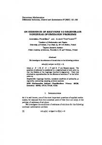
Global Optimization Due to the scale of water networks of interest in practice, both VP-MINLP and VS-NLP are of challenging dimension for global solvers of non-convex optimization problems. The limitations of current global solvers for design decision problems have been discussed by Bragalli et al. (2011) and Eck and Mevissen (2012). Recent progress for some operational decision problems has been reported in Gleixner et al. (2012). Since VP-MINLP and VS-NLP are polynomial optimization problems of degree three we take advantage of the hierarchy of semidefinite programming (SDP) relaxations pioneered in Lasserre (2001), in order to (a) derive global lower bounds for the optimal value of VP-MINLP and VS-NLP; and (b) approximate the global optimal solution of VS-NLP for the case where VS-NLP has a unique global optimizer. The derived lower bounds are used to examine the global optimality gap of the local solutions obtained by Bonmin and Ipopt. Furthermore, in the case VS-NLP has a unique global optimizer, the approximation for the global optimizer obtained from solving the SDP relaxation can be used as a starting point for a local optimization method such as IPOPT. Making the SDP relaxation increases the size of the global optimization problem, but this size can be reduced substantially if the underlying polynomial optimization problem is sparse, i.e. having a small number of variables in each constraint only, as proposed by Waki et al. (2006). Many real-world water networks can be represented by sparse graphs because the degree of most nodes in the networks is small. The sparsity of a water network results in VS-NLP being a sparse polynomial optimization problem. In order to exploit this sparsity and solve the sparse hierarchy of SDP relaxations of Waki et al. (2006), we use SparsePOP (2012) with SDPA (2012) as the SDP solver. RESULTS AND DISCUSSION The methods described above are applied on the ”Pescara” water network, which is a reduced version of a network for a medium size Italian city. The network is first mentioned by Bragalli et al. (2011), who also make available online the model file in Epanet format. Computations were performed running Red Hat Linux on a blade server with with 100GB (total, 80 GB free) of RAM and a processor speed of 3.5GHz. Local solver The results for applying Bonmin B&B to optimally place 1-4 PRV can be found in Table 1. In making the model runs, the minimum pressure was set at pmin = 19m as this was the lowest pressure in the system before placing valves. As expected, placing additional PRVs reduces the objective value but increases the computational time. Note the diminishing returns for placing additional valves in terms of additional pressure reduction. Optimal locations for 2 new PRVs are shown on the network map (Fig. 1). This network has several loops and so is a nice illustration of the utility of optimization methods for supporting design decisions. It is not obvious from the 5
TABLE 1. Computational experience for the valve placement problem on the Pescara network of Bragalli et al. (2011) having 76 nodes and 99 pipes (see Fig. 1). Valves to place 0 1 2 3 4
Run Objective Marginal Time (s) value Reduction 2 2013 25 1867 7.3% 623 1764 5.5% 1167 1749 0.9% 5522 1734 0.9%
Total Reduction 7% 12% 13% 14%
FIG. 1. Pescara network due to Bragalli et al. (2011) with two pressure reducing valves placed in optimal locations as found in the present paper. Elevation contours shown in the figure are computed from nodal values.
network topology and elevations where valves should be placed. With the optimal placement of two values, a pressure reduction of 12% is achieved. Assuming that leakage is directly proportional to pressure (see Lambert (2001)), this pressure reduction corresponds to approximately a 12% reduction in leakage. Comparisons between the flow and pressure solution derived by the optimization model were compared with those obtained by EPANET for the two valve case to assess the accuracy of the quadratic approximation. Results showed that solutions computed using the approximation are consistent with Epanet (Fig. 2). 6
60
200 ● ● ● ●
●
● ● ●
●
100
● ● ●
Bonmin Flow (L/s)
Bonmin Pressure (m)
●
● ● ● ● ● ●● ● ●
30 ●● ● ● ●● ● ● ● ●● ● ● ● ● ● ● ● ● ● ● ● ● ●● ●
● ●● ●● ● ● ● ●● ● ● ● ● ● ● ● ● ● ● ● ● ● ● ● ● ● ● ● ● ●
0 ● ● ●● ● ● ●
−100 (b)
(a) 0
●
0
30 EPANET Pressure (m)
●
60
−100
0 100 EPANET Flow (L/s)
200
FIG. 2. Comparison of pressures (a) and flows (b) for the Pescara network as calculated by Bonmin with quadratic head loss and EPANET 2.0.
Global solver The VS-NLP for Pescara network satisfies a correlative sparsity pattern (Waki et al. 2006) as illustrated in Fig. 3, left. The chordal extension of this pattern (Fig. 3, right) is exploited by SparsePOP to form a sparse SDP relaxation for VS-NLP. We consider the VS-NLP for optimally setting the 2 PRVs on pipes ’90’ and ’97’ obtained by Bonmin, and solve the SDP relaxation of order 2, which is the lowest order relaxation for VS-NLP. Table 2 contains the lower bound given by the minimum of the SDP relaxation, the IPOPT solution and the relative gap between the two. Thus, the lower bound obtained from the SDP relaxation for the global optimum of the VS-NLP provides a performance measure for the local method described above. For the zero valve case of VS-NLP, the optimization problem is equivalent to the network simulation problem of finding the distribution of flows and pressures. Indeed, the solution obtained by simulation is identical to that obtained from both local and global optimizaitons. The result that global and local solutions coincide can be explained by the fact the simulation problem has a unique solution. To see that the solution to a network simulation problem is unique, Berghout and Kuczera (1997) argue that a network comprised of links with ’strictly convex content’ can be posed as a convex optimization problem, a result due to Collins et al. (1978). Since Pescara lacks non-convex elements, such as pumps, the feasible flow and pressure solution is unique and may be found by simulation, local optimization, and global optimization. Where settings for 1 or more PRVs are required, there are infinitely many feasible solutions. For the scenarios considered here, the local solver found solutions with relative global optimality gaps of less 7
0
0
50
50
100
100
150
150
200
200
250
250 0
50
100
150 nz = 3007
200
250
0
50
100
150 nz = 15165
200
250
FIG. 3. Correlative sparsity pattern (left) and chordal extension for the correlative sparsity pattern (right) for VS-NLP. TABLE 2. Comparison of global and local solutions for the valve setting problem (VS-NLP) on the Pescara network. Num. valves to Set 0 1 2
Global Global Lower Run Local Bound Time (s) Soln. 2013 10,974 2013 1744 16,014 1867 1669 15,367 1764
Local Relative Run Gap Time (s) 0.0% 2 7.1% 2 5.7% 3
than 10% in a short time. CONCLUSION This paper has applied local and global optimization methods to the problem of pressure management on water networks. Formulation as a polynomial optimization problem enables solutions using both local and global methods. In the experiments reported here, the local solutions to the valve setting problem had a small optimality gap when considering the run time of the global method was at least three magnitudes larger than the local one.
8
Notation a b di ei hf vi,j A−E C D L Nn Np Nv Q Q1 Q2 V α
dimensional coefficient, dimensional coefficient, water demand at node i, elevation at node i, frictional head loss [m], valve indicator, constants used to compute a and b for Hazen-Williams, Hazen-Williams C-value, Pipe diameter [m], Pipe length [m], Number of nodes in the network, Number of pipes in the network, Number of valves in the network, Flow rate [m3 /s], Flow rate at lower end of approximation interval [m3 /s], Flow rate at upper end of approximation interval [m3 /s], Average fluid velocity [m/s], Constant part of Hazen-Williams formula
REFERENCES Bonmin (v. 1.5) (2011), . Ipopt (v. 3.10) (2011), . SDPA-M (v. 7.3.6) (2012), . SparsePOP (v. 2.99) (2012), . Berghout, B. L. and Kuczera, G. (1997). “Network linear programming as pipe network hydraulic analysis tool.” Journal of Hydraulic Engineering, 123(6). Bragalli, C., Ambrosio, C. D., Lee, J., Lodi, A., and Toth:, P. (2011). “On the optimal design of water distribution networks: a practical minlp approach.” Optim. Eng. Collins, M., Cooper, L., Helgason, R., Kennington, J., and LeBlanc, L. (1978). “Solving the pipe network analysis problem using optimization techniques.” Management Science, 24(7), 747–760. Eck, B. J. and Mevissen, M. (2012). “Valve placement in water networks: Mixed-integer non-linear optimization with quadratic pipe friction.” Report No. RC25307 (IRE1209-014), IBM Research (September). Gleixner, A., Held, H., Huang, W., and Vigerske, S. (2012). “Towards globally optimal operation of water supply networks.” Numerical Algebra, Control and Optimization, 2(4), 695–711. Hindi, K. S. and Hamam, Y. M. (1991). “Locating pressure control elements for leakage minimization in water supply networks: An optimization model.” Engineering Optimization, 17(4), 281–291. Lambert, A. (2001). “What do we know about pressure:leakage relationships in
9
distribution systems.” IWA Conference System Approach to Leakage Control and Water Distribution Systems ManagementISBN 80-7204-197-5. Lasserre, J. B. (2001). “Global optimization with polynomials and the problem of moments.” SIAM J. Optim., 11(3), 796–817. Nicolini, M. and Zovatto, L. (2009). “Optimal location and control of pressure reducing valves in water networks.” Journal of Water Resources Planning and Management, 135(3), 178–187. Rossman, L. A. (2000). Epanet 2 users manual. US EPA, Cincinnati, Ohio. Sherali, H. and Smith, E. (1997). “A global optimization approach to a water distribution network design problem.” Journal of Global Optimization, 11, 107– 132. Waki, H., Kim, S., Kojima, M., and Maramatsu, M. (2006). “Sums of squares and semidefinite program relaxations for polynomial optimization problems with structured sparsity.” SIAM J. Optim, 17, 218–242.
10