region, the Gauss-Newton algorithm may not converge since known estimates of the ..... 0k(n) =[ark(n) 02k(n) bok(n) bik(n)]T with k = 1, 2,. , N/2 â 1. In all cases ...
IEEE TRANSACTIONS ON CIRCUITS AND SYSTEMS—II: ANALOG AND DIGITAL SIGNAL PROCESSING, VOL. 41, NO. 8, AUGUST 1994
561
Transactions Briefs Fast Parallel Realization of IIR Adaptive Filters
Paulo S. R. Diniz, Juan E. Cousseau, and Andreas Antoniou Abstract— A parallel realization based on the voltage-conversion generalized-immittance converter is used for the implementation of adaptive HR filters. Through this approach, the convergence rate of the parallel realization is substantially increased, and becomes comparable or higher than that in the direct-form realization and much higher than that in the lattice realization. The paper deals with the reasons that lead to the improved performance and provides extensive experimental results that illustrate the fast convergence, reduced computational complexity, and improved robustness. I. INTRODUCTION
In certain applications an adaptive filter is required that will adjust its transfer-function coefficients to match those of an unknown system. For this task IIR adaptive filters have certain advantages over corresponding FIR filters. IIR adaptive filters require less computation and can model sharp resonances more easily. However, the requirement of monitoring filter stability, the slow convergence, and the possibility that the mean-square-error (MSE) surface may have multiple local minima that may prevent the filter from converging to an acceptable solution have prevented the widespread use of these filters. The choice of realization influences the convergence rate, the computational complexity of the gradient vector, the stability monitoring [1], [2], and the shape of the MSE surface [1]; however, it cannot prevent unacceptable local minima. The parallel form is an attractive realization for the implementation of IIR adaptive filters because stability can be easily monitored and the gradient vector can be efficiently computed. However, since the interchange of sections does not alter the overall transfer function, a number of equivalent global minimum points located in distinct subregions of the parameter space are possible. The subregions are separated by boundaries that represent reduced-order manifolds [1]. These boundaries contain saddle points and if the initial point is assumed to be in such a region, the convergence rate is usually low. On the other hand, if the solution point approaches a boundary region, the Gauss-Newton algorithm may not converge since known estimates of the cross-correlation matrix, designated as R, can become ill-conditioned [3]. It has been suggested in the literature that the parallel realization leads to slower convergence than the direct-form and lattice realizations [I], [6]. However, as will be demonstrated in this paper, by appropriately configuring the parallel realization, the rate of convergence increases to a level that is as high as, if not higher than, that in direct-form and lattice realizations. An attempt to improve the performance of the parallel realization has been first described in [3] and further extended in [4], [5] Manuscript received February 15, 1993; revised November 24, 1993. This paper was recommended by Associate Editor G. S. Moschytz. P. S. R. Diniz and J. E. Cousseau are with Prog. de Engenharia Eletrica e Depto de Eletronica COPPE/EE/Federal University of Rio de Janeiro, Rio do Janeiro, R.J., Brazil 21945. A. Antoniou is with the Dept. of Electrical and Computer Engineering University of Victoria, Victoria, BC, Canada, V8W 3P6. IEEE Log Number 9402396.
for filters with real coefficients. In this approach a prefilter is incorporated at the input of the parallel form. The prefilter is implemented with the discrete Fourier transform and generates m signals that are individually applied as inputs to first-order complex sections. With this strategy, an estimate of matrix R, designated as R(n ), is less likely to become ill-conditioned. In addition, a gradient-type algorithm is less likely to get stuck in a reducedorder manifold. However, the use of preprocessing increases the computational complexity. The approach leads to faster convergence but the performance of the direct-form and lattice realizations has not as yet been matched. In this paper, a parallel realization based on the voltage-conversion generalized-immittance converter (TVGIC) [7] is used in the implementation of adaptive filters. In this approach, the gradient vectors of the various sections are different even if the poles of the sections are located at the same position. This tends to reduce the number of iterations needed by the algorithm to escape from boundary regions. In a sense, the function of the prefilter is performed by the parallel sections themselves without the use of a prefilter. This strategy yields filters that outperform the filters in [3], as has already been demonstrated in [8]. The paper presents, in addition, an error surface analysis that helps one understand how the configuration strategy of the parallel realization works. Experimental results obtained confirm the improved performance of the proposed realization. II. NEW PARALLEL REALIZATION
A widely used adaptation algorithm involves the use of the Gauss-Newton algorithm for the minimization of the mean-square error (MSE) defined as MSE =
Efe2 (01 = E{[d(n)
-
y(n)]2}
where y(n) is the output signal, e(n) is the error signal and d(n) is the reference signal. The updating of the coefficients can be performed as e(n + 1) = e(n) + „P(n 1)*(n )e(n) where 6)(n)
= Vg(n) 8I(n)
••• 0
(r1)11
is the coefficient vector, (T) = V y(n)
is the gradient vector with respect to the coefficients, convergence factor, and P(n + 1) = P(n + 1)
is the
(n 1).
is obtained through the following recursive relation
1 [ 1-„ i , P(n +1) = 1 ,"11 a„
P(n)W(n)cT (n)P(n) 1 - 1 +W I' (n)P(n)W(n) a„ -
The value of the convergence factor affects the performance of the parallel realization critically; for example, if the current parameter estimate moves into a reduced-order region of the MSE surface [1],
1057-7130/94504.00 © 1994 IEEE
562
IEEE TRANSACTIONS ON CIRCUITS AND SYSTEMS—II: ANALOG AND DIGITAL SIGNAL PROCESSING, VOL. 41, NO. 8, AUGUST 1994
(a) y011
106 tpftn) 422(n) 1700 hp1(n) hp2(n)
(b) Fig. 1. (a) TVGIC structure; (b) TVGIC block representation.
a large step size would cause the parameter estimate to move away from this region of ill-conditioning. An estimate of the information cross-correlation matrix R = EIW(n)e(n)} is given by [9] R(n + 1) = (1 — n)R(n) + ckW(n)Wil (n)
where W(n) is the gradient vector. For large n [3]
E(1 - cx)'#(n — /)e(n
R(1). ± 1)
—1).
i=o
As the individual sections tend to become identical in the parallel form, matrix R(n + 1) tends to become singular because W(n — 1)*ri(n — 1) has a block structure with each block having identical elements [3]. This can lead to slow convergence and possibly to lack of convergence. The task of keeping the partial derivatives different from coefficient to coefficient can be accomplished by choosing a set of distinct parallel sections for the realization of the adaptive filter. A general digital-filter configuration that realizes several types of biquadratic transfer functions simultaneously at no additional cost is the transposed VGIC (or TVGIC) structure depicted in Fig. 1 [7]. The available transfer functions are given by
(z +1)2 H151 (Z) =
D(z)
11(p2 (Z) =
(z —1 )= ,111,2(z) — D(z) )
(z + I) D(z) (z _ 1) 2
ilbp( 2 )
( z2— 1) D(z)
D(z)
where D(z) = z 2+ (ml — m2)z + m + m2 —1
and the subvectors of
Fig. 2. Parallel TVGIC realization of 10th-order filter.
highpass outputs, respectively. A specific arrangement for a tenthorder adaptive filter is depicted in Fig. 2. If the multipliers m,, are all different from zero, then each filter is a distinct section and the arrangement may be deemed to be a filter bank. The partial derivatives of the transfer function with respect to the multiplier coefficients are forced to be different even when some of the poles of the sections coincide. The exception is that the partial derivatives with respect to numerator multiplier coefficients, i.e., m„, for j > 3, coincide if the poles in these sections coincide. This could cause the matrix R(N + 1) to become singular. However, this will most probably not occur in the next step because the poles in these sections are updated differently. An alternative approach to reduce the likelihood of R(n +1) from becoming singular is to create alternative outputs for the TVGIC sections by adding and subtracting pairs of the available outputs, and to ensure that all sections use different outputs. This approach should be used if, for example, a sixth section is needed in Fig. 2. A rule to specify the outputs of the sections is that each of them must have a distinct combination of outputs, for example, if two outputs are chosen for a given section these two cannot appear simultaneously as the outputs of any other section. This rule guarantees that the poles in each section are updated differently if they happen to coincide at a given iteration. It should be mentioned that a number of alternative general digital-filter configurations that realize several types of biquadratic transfer functions simultaneously have been reported in the literature [10]—[14], which are good candidates for the second-order sections in the parallel form. We have chosen the TVGIC structure because of the reduced number of additions required and the simplicity of gradient computation.
(n) are given by III. GRADIENT COMPUTATION
9, ( 7
) = [rn 1) met m3, mt, zn5,] T .
Distinct sections can be obtained by forming linear combinations of two or more of the outputs of the TVGIC structure illustrated in Fig. 1, where 1pi(n), hpi(n), and bp(n) represent lowpass, bandpass and
Assuming that the adaptive transfer function is varying slowly, the gradient components can be calculated by using the derivatives of the transfer function with respect to the multiplier coefficients [2] at instant n. For a general structure, the required partial derivatives can
IEEE TRANSACTIONS ON CIRCUITS AND SYSTEMS—II: ANALOG AND DIGITAL SIGNAL PROCESSING, VOL, 41, NO 6, AUGUST 1994
x(rt)
Fig. 3. Gradient calculation.
be approximated as [15] 2{:mY ( nn),) ]
Hi, j (z)H.,,2(z)X(z)
where H1,3 ( z) is the transfer function from the filter input to the input of multiplier m,( k), and /1j,2(Z) is the transfer function from the multiplier output to the filter output. In the case of the TVG1C structure, the multipliers not belonging to the recursive part are incident to the output node such that H,,2(z) = 1 and H1,3 (2)X(z) is available in a parallel realization. The multipliers belonging to the recursive part of the structure are incident to the input node such that Z
ay( n) R.. - H1 1,(z)H,(z)X(z) ' Ln] atnii( )
for I = 1, 2, where H,(z) is the transfer function of the ith section. Since Hi (z)X( a) is also available in the parallel realization, only one additional TVGIC block per section is required to calculate the derivatives, as illustrated in Fig. 3. It should be mentioned that under the assumption of slow parameter variation, any structures with all the multipliers incident to the input and output nodes will lead to efficient gradient computation. Since the TVGIC structure is, in addition, canonic with respect to the number of multipliers, the resulting realization has reduced computational complexity, and is competitive with direct-form realizations. Furthermore, stability monitoring is simple. IV. A STUDY OF THE MSE SURFACE
The purpose of this section is to provide, through the analysis of the MSE surface, an interpretation for the advantages of TVGIC over direct-form sections. It is well known that the MSE performance surface of a direct-form adaptive IIR filter can have local minima [16]. This characteristic is a result of the feedback that causes the filter output to be a nonlinear function of the coefficients. The Gauss—Newton minimization algorithm could converge to any of these minima thereby resulting in suboptimal performance. This disadvantage is a characteristic of IIR adaptive filtering, and is generally unavoidable except under special circumstances. One such case, is in a system identification application where it is possible to have a global minimum without any local minima [17] if the adaptive filter is of sufficient order and the number of coefficients in the numerator of the transfer function of the adaptive filter is larger than the order of the denominator of the transfer function of the unknown system. In the following discussion, it is assumed that the adaptive filter is modeling an unknown system and that the MSE surface of the direct form has a single (global) minimum.
563
Among the alternative realizations for IIR adaptive filters, the parallel structure represents an efficient one in terms of computational complexity; however, it does not have a unique representation. The parallel form is obtained by expressing the transfer function as the sum of V/2 second-order sections and by reordering these sections as many as (N/2)! different realizations can be obtained. For a parallel structure comprising direct-form second-order sections it is important that the coefficients be initialized such that the sections have different paths of evolution during the adaptation. This prevents the estimated Hessian matrix in the Gauss—Newton minimization algorithm from becoming ill-conditioned. This problem can occur each time the gradient vector contains some identical elements. It has been shown, however, that the condition of identical sections corresponds to reduced order manifolds [1] on the MSE surface, a region of the parameter space where the convergence rate is extremely slow. In a parallel realization with TVGIC second-order sections, the convergence rate reduction is avoided if the sections are forced to be different. In order to illustrate the ability of a TVGIC-based realization to avoid the manifolds associated with the parallel structure during adaptation, an analysis of the gradient vector behavior in the neighborhood of a reduced order manifold is first provided. A. Gradient Vector Behavior
We will now show that if two distinct sections of the parallel realization have poles close to each other, the TVGIC-based realization tends to update the parameters in such a way that the poles move away from each other. On the other hand, in the standard parallel realization with direct-form sections, the pole positions tend to remain close to each other after the updating of the coefficients. These statements are substantiated by the following discussion. Assume that in a given iteration the poles of two distinct sections i and j are close to each other and let the respective denominator polynomials be D1(z) = z2 + al, 0.2, and ./),(;) = z + (al r Xl).Z. (aa, + A2). The gradient vector for any parallel realization is of the form
)
= [COO • C(n) •
*)(n)
... *Al2-1(ne
where W,(//) = V 9y(n) is a subvector that corresponds to the gradient of the filter output with respect to the coefficients of section i. In the following analysis, *d (n) and IP'(a) represent, respectively, the gradient vectors for the direct-form and TVGIC-based parallel realizations. For a parallel realization with direct-form sections, the difference between the gradient subvectors of two distinct sections is given by
AC (n) = (12 ) — *'1(m) .
(n)
Dj (z) '(n) D., (z) •T( 11 )
Di(z) x(n)
Dj(z) x(n) Di(z)
564
IEEE TRANSACTIONS ON CIRCUITS AND SYSTEMS—II: ANALOG AND DIGITAL SIGNAL PROCESSING, VOL. 41, NO. 8, AUGUST 1994
- 2Bi(z) z
D? (z)
2B,(z)
D,(z)
In these expressions, N1, (z) is the numerator of the lth output of the ith section in the parallel realization, i.e.,
(Aiz + A2)x(n)
(Aiz + A2)x(n)
(z) = 4,22 ±
2
z A2)x(n)
D,(z)
Di(z 1
(
N2, (Z) 74,22 +nzaz + nzi
B,„(z)-= m 3,No,(z)± 7n4,N1,(z)-1- rr15/V21(z)
(Ai z A2)x(n)
where the zeros have been considered coincident, and the following approximation has been employed
Thus, for Al and A2 > 0, the gradient subvectors of distinct sections always point to different directions. Furthermore, this conclusion applies even if the zeros of sections i and j coincide. Therefore, in a TVGIC-based realization the solution point can easily move away from a reduced-order manifold.
1
1 _ Di(z) z2 + 1
B. Positive Definiteness of the Covariance Matrix
+ (a2 + A2) ,A1Z ± A2 D,(z)
Di (2)
1 D,1(z)
1 OD,(z)
At z
By denoting the covariance matrices of the parallel realizations using the TVGIC and direct-form sections as Ri (n) and Rd(n), respectively, we can write
,A2) 2
Di (z) )
1
2 ( A z ± A2)
DF(z)
M(z)
Rt (n) = Eltft (re)c' T (n)}
where
As can be observed, when the coefficients of the sections approach each other (i.e., as Ai, A2 tend to 0), the gradient subvectors of sections 1 and j tend to point in the same direction. Since small convergence factors are usual in IIR filters, any two sections that have similar coefficients will continue to have similar coefficients over a number of iterations thereby delaying convergence. For the TVGIC-based parallel realization the difference between the gradient subvectors of two different sections is given by
= [# o (n)
(n) -
Rd(n) = Elf d (n)W dT (n)}
where #d (n) WOO
(z
D,(z)
— (z + 1)
:0(n)
(z
D,(z)
1)
D())
1)
-Aq,31
Dj(z)
xnj(n)
D,(z) ri,(n) D,(z) x 2,(n) D,(z)
D3(z)
Rt(n) = TRd(n)TT
ACJ2 (2)
Ax11,,3
(n) D,(z)
A 'Fq.j1
x23 (n)
A~Yiis
D,(z)
1-2(Boi(z)— Bo,(z))(A1 D; (z)
ix(n)
N2j
x(n)
0
TA12-1
-1 —1 0 0 0 —1 —1 0 0 0 Ti = 0 0 not not 0 0 n11n7; 74; _ 0 0 4i
(z — 1)
Adx(n)
Using Theorem 8.1.12 of [18], it is easy to conclude that
41. > + A2 dx(n)
NIA() — Nii(lx(n) [D,j((z))(Alz A2)1x(n) z)
0
and
12(Boi(z)— Boi(z)) (A1 z A2 )] x (n) D?(z) A+,33= [Noi(zrzN)oi(z)] x(n)± .N D -0:((zz))
rAr2i (z)—
To
-
Allri • = —(z + 1)[ 19'" (z .(z B"(z) ]x(n) — (z +1)
[
where T=
where ()
esr/2-1(71)1T -
With Cl (n) defined in (1) it can be easily shown that
-
b(n)
xo,(n)
A1Yzi1 = (z 1) roi(z) —(z)
N/ 2-1 )1 T
•
with C(n) defined in (2), and
A*1, j(n) = 4P(n) —*;(n) (z — 1)
2
)
A2)x(n)
)(Alz
D,(z)
+ 72,2, + n1 ,z+
Ni,(z)= 7101i 22 +
{ D2i: )) (AI Z A2)]x(n)
m
„,„ are the minimum eigenvalmt„, am n , and )Q where Q = ITT , AR ues of matrices Rt(n), Rd(n), and Q, respectively. Usually A„ Q „., > 2 and as a result the covariance matrix for the TVGIC realization is more likely to remain positive definite. In particular, for a fourth-order adaptive filter with the TVGIC outputs chosen as ipl, by and /tp2 for section 1 and bp, ipl and hp2 for section 2, we have A21, = 2. Therefore, Aal >
IEEE TRANSACTIONS ON CIRCUITS AND SYSTEMS—II: ANALOG AND DIGITAL SIGNAL PROCESSING, VOL. 41, NO. 8, AUGUST 1994
565
V. SIMULATION AND COMPARISONS
In order to test the use of TVGIC sections in the implementation of IIR adaptive filters, several adaptive filters were simulated employing different realizations. The experimental setup consisted of system identification applications with a white noise signal of unit variance as input and a measurement white noise which was uncorrelated with the input signal. The MSE learning curves were obtained by averaging the squared error from 25 independent computer runs. In addition to the TVGIC parallel realization, the following realizations were used for the IIR adaptive filter: • Direct-form realization y(n)
= E bk(n)x(n — k)
E
k,0
-15.0
-45.0
a k (n)y (n. — k)
k=1
where the coefficient vector is % 00
e(n) = [a l (n) •
aN(n) bo (n) • • • b N ( n )r
4000.
400.0
Fig. 4. MSE learning curves for fourth-order system. (a) Direct form. (b) Parallel structure with direct-form sections. (c) Parallel structure with TVGIC sections.
• Lattice realization y(n) = Ik o a k(n)bk(n) f N (n) = x(n) f k (n) = f k (n) — pk(n)bk_ 1 (71 — for k = 1, 2, - , N
1)
bo(n) -=- fo(n) bk(n) = bk _ i (n — 1) + pk(n).6.--1 (n) for k = 1, 2, • • • , N
where the coefficient vector is e(n) = [pi (n) •
p (n) Ao(n) • • AN (n)1T
• Parallel realization with direct-form sections y(n) = Eikv=lg Yk( 21) yo(n) = E,2,,_,b„,o (n)x(n — m)
▪ Elm_ amo (n)yo (n — m) =0 bmk (n)x(n — Tn)
Yk(n) =
▪ E 2m -i amk(n)yk(n - rn) for
k=1 ,• • • ,
N/2-1
The coefficient vector for this case is e(n) = [07;(n) • • •
Fig. 5. MSE learning curves for fourth-order system. (a) Direct form. (b) Parallel structure with TVGIC sections. (c) Parallel structure with identical direct-form sections. (d) Parallel structure with different direct-form sections.
OTT/2-1 (Ti)]T
where for section 0, realization with TVGIC sections has a performance close to that of the direct-form realization. In the second set of simulations, the transfer function of the system to be identified was z(z — 0.9)(z2+ 0.81) 11(z) = 2 (z — 0.71z + 0.25)(z2 + 0.75z + 0.56)
00(n) = [aio(n) a20(n) boo(n) bio (n) b20 (n)]T
and for section
k,
0 k(n) =[ark(n) 02k(n) bok(n) bik(n)] T
with
k = 1,
2,
, N/2 — 1.
In all cases, the gradients were computed using the assumptions discussed in Section III. In the first set of simulations, the transfer function of the system to be identified was H (z) =
(z 2—
(z — 0.9)(z 2+ 0.81) 1.13z + 0.64)(z2 + 0.9z + 0.81) .
(3)
The realizations compared were the parallel realization with TVGIC and direct-form sections, and the direct form. In each case, the convergence factor was a = 0.01, and v(n)) was a zero-mean process with variance —32 dB. To avoid the basic problem of starting in a manifold of the parallel realization, the poles of all the realizations were initialized at pk = Lkr rI4, k = 1, • • • , N for r = 0.01. The chosen outputs of the TVGIC sections were by and 1p2 for section 1; and bp, hpl and hp2 for section 2. The learning curves are shown in Fig. 4, and as can be observed the parallel
In these simulations v(n) was set to 0 and the initialization was the same as in the previous example. The learning curves are shown in Fig. 5. For the sake of comparison, the MSE learning curve of the parallel realization with direct-form sections with two numerator coefficients in the first section and three numerator coefficients in the second section is also included. This realization can avoid reducedorder manifolds but since the number of parameters of the overall numerator is five, convergence is slower than for a parallel realization with four numerator coefficients. In the third set of simulations the transfer function to be identified was 2.3 (z — 0.9) H(z) — (z 2— 0.71z + 0.25)(z2 +0.75z + 0.56) (z2 + 0.81)
(z2— 0.22 + 0.81)•
566
IEEE TRANSACTIONS ON CIRCUITS AND SYSTEMS—IL ANALOG AND DIGITAL SIGNAL PROCESSING, VOL. 41, NO. 8, AUGUST 1994
Condit ion Hunter
4000.
No . of iterations - 12O b 00
1600.
3300.
4000.
6400.
11 00
Fig. 6. MSE learning curves for six-order system. (a) Direct form. (b) Parallel structure with TVGIC sections. (c) Parallel structure with direct-form sections.
TABLE I CONVERGENCE SPEED COMPARISONS Realization Type of filters Parallel realization
Number of iterations Lowpass
Highpass
Bandpass
3375
2713
2278
with TVGIC-form sections
1087
1104
1240
Direct-form realization Lattice-form realization
1066 2107
947 1546
1461 2052
with direct-form sections Parallel realization
In this case v(n ) and the initialization were the same as before. The chosen sections for the parallel TVGIC realization were 1pl and 1p2 for section 1; 1p2, by and hp2 for section 2; and hpl and hp2 for section 3. The MSE learning curves are depicted in Fig. 6. Finally, a comparative study has been undertaken and the results obtained are summarized in Table I. In this study, several adaptive filters were simulated using (a) the parallel structure with direct-form sections (b) the parallel structure with TVGIC sections, (c) the directform realization, and (d) the lattice realization. The systems to be identified were lowpass, highpass and bandpass Chebyshev filters of sixth-order, v (n) was a white-noise process with variance -40 dB, and a = 0.01. The initialization used previously was employed in all filters. Convergence was assumed to have been achieved when the average square error of the last 200 samples reach a level below -35 dB. The chosen outputs of the TVG1C structure were by and 1p2 for section 1; 1p2, hp, and h.pl for section 2; and by and hpl for section 3, for the lowpass and bandpass filters. For the highpass Chebyshev filter, the outputs used were by and for section 1; 1p2, hp and hpl for section 2; and by and hp2 for section 3. As can be seen in Table 1, the proposed realization always leads to fast convergence which is comparable to that of the direct-form realization. These results confirm the good performance of the direct-form realization, as is already well known. The new parallel realization is also more robust than the direct-form based parallel realization since it maintains a better conditioning on matrix P (n) during the adaptation process. This attribute can be noted in Fig. 7 for the case of the identification of the system described by (3) and was noted in all examples tried out.
900.0
4900.
1000 .
Fig. 7. MSE condition number of matrix P(n). (a) Parallel TVGIC realization. (b) Parallel direct-form realization.
VI. CONCLUSIONS A technique that improves the convergence rate in the parallel realization of adaptive HR filters has been proposed. The technique involves keeping the gradient vectors of the various sections different by using a suitable parallel realization based on the voltageconversion generalized-immittance converter in the implementation. A study of the error surface has shown that different error surfaces are obtained with respect to the filter coefficients. This feature enables the solution point to move away from boundary regions and, consequently, results in fast convergence in the adaptive filter. It also leads to improved robustness by maintaining a better conditioning on the cross-correlation matrix. The expected improvement in the adaptation process has been demonstrated by extensive experimental results and simulations. REFERENCES M. Nayeri and K. Jenkins, "Alternate realizations to adaptive IIR filters and properties of their performance surfaces," IEEE Trans. Circ. Syst., vol. 36, pp. 485-496, Apr. 1989. J. J. Shynk, "Adaptive IIR filtering," IEEE Acoust., Speech, Signal Processing Mag., vol. 2, pp. 4 21, Apr. 1989. J. J. Shynk, "Adaptive BR filtering using parallel form realizations," IEEE Trans. Acoust., Speech, Signal Processing, vol. 37, pp. 519-533, Apr. 1989. H. Perez and S. Tsujii, "A fast parallel form IIR adaptive filter algorithm," IEEE Trans. Signal Processing, vol. 39, pp. 2118-2122, Sept. 1991. P. S. R. Diniz, J. E. Cousseau, and A. Antoniou, "Improved parallel realization of RR adaptive filters," Inst. Elect. Eng. Proc. Circuits, Devices and Sytems, pt. G, vol. 140, pp. 322-328, Oct. 1993. J. J. Shynk, "Performance of alternative adaptive IIR filter realizations," in Proc. 21 st Asilomar Conf. Signals, Systems, Computers, Pacific Grove, CA, 1987, pp. 144-150. P. S. R. Diniz and A. Antoniou, "Digital-filter structures based on the concept of the voltage-conversion generalized immitance converter," Can. J. Elect. & Comp. Eng., vol. 13, pp. 90-98, Apr. 1988. P. S. R. Diniz, J. E. Cousseau, and A. Antoniou, "Fast adaptive IIR parallel realization," in Proc. IEEE Int. Symp. Circ. Syst., San Diego, CA, 1992, pp. 2200-2223. L. Ljung and T. SOderstrom, Theory and Practice of Recursive Identification. Cambridge, MA: The MIT Press, 1983. P. S. R. Diniz and A. Antoniou, "On the elimination of constant-input limit cycles in digital filters," IEEE Trans. Circ. Syst., vol. 31, pp. 670-671, July 1984. H. Kwan, "A multi-output second-order digital filter without limit cycle oscillations," IEEE Trans. Circ. Syst., vol. 32, pp. 974-975, July 1985. -
IEEE TRANSACTIONS ON CIRCUITS AND SYSTEMS—II: ANALOG AND DIGITAL SIGNAL PROCESSING, VOL. 41, NO. 8, AUGUST 1994
[12] —, "A multi-output wave digital biquad using magnitude truncation instead of controlled rounding," IEEE Trans. Circ. Syst., vol. 32, pp. 1185-1187, Nov. 1985. [13] C. Eswaran, A. Antoniou, and K. Manivannan, "Universal digital biquads which are free of limit cycles," IEEE Trans. Circ. Syst, vol. 34, pp. 1243-1248, Oct. 1987. 114] T. Kwan and K. Martin, "Adaptive detection and enhancement of multiple sinusoids using a cascade HR filter," IEEE Trans. Circ. Syst., vol. 36, pp. 937-947, July 1989.
567
[15] A. Antoniou, Digital Filters: Analysis, Design, and Applications, 2nd ed. New York.: McGraw-Hill, 1993. [16] S. D. Stearns, G. R. Elliott, and N. Ahmed, "On adaptive recursive filtering," in Proc. 10th Asilomar Conf. Signals, Syst., Computers, Pacific Grove, CA, 1976, pp. 5-10, 1976. [17] T. SOderstrom, "Some properties of the output error method," Automatica, vol. 18, pp. 93-99, Jan. 1982. [18] H. Golub and C. VanLoan, Matrix Computation. Baltimore, MD: The Johns Hopkins Univ. Press, 1987.
r17:7C-Zi2