that, if one wishes to know the force exerted on an apple by the. 1050 atoms in the ..... mass of a typical galaxy (1011â1013 solar masses). To gen- erate data sets ..... Figure 10: Time per timestep for the vortex method vs. number of vortices ...
Fast Parallel Tree Codes for Gravitational and Fluid Dynamical N-Body Problems
provide a method of computing the mutual interactions of N bodies in much less than O (N 2 ) time. Tree codes have been reported to scale as O (N ) or O (N log N ), but the “big-O” notation can be misleading for practical values of N , where true performance is dominated by the constants that are discarded by the asymptotic analysis. Large-scale application of tree-based approximation methods has (to our knowledge) only occurred in astrophysics, [41, 16, 40, 24] although preliminary work has been done on two-dimensional [33, 31, 21, 19], and three-dimensional systems [22, 39, 8, 15] from other disciplines. One roadblock to the widespread acceptance of tree codes is that they are inherently complex to program, especially for parallel machines. We report on an implementation of a tree code which is not specific to a particular problem domain. Although designed with astrophysical research firmly in mind, the code described here is used to address example problems in vortex dynamics as well as astrophysics. We report on its performance on the Intel Touchstone Delta system with up to 512 distributedmemory processors. Two outcomes are possible when algorithmic advances drastically reduce the time and space required to solve a class of problems. The first is that the problems cease to be “supercomputer applications”, and fall into the domain of workstations and personal computers. The second is that practitioners gradually advance the state-of-the-art in the underlying discipline, and much larger problems become the norm. In the latter case, supercomputers remain a critical component, and it is important to address issues of whether the new algorithm is well-suited to supercomputer architectures, i.e., massively parallel systems. The second outcome has certainly been the case in astrophysics, where state-of-the-art simulations now evolve systems of 107–108 bodies. We expect it will occur in other fields as tree-based methods become generally available.
Submitted to the International Journal of Supercomputer Applications. Accepted for publication in Vol 8.2.
John K. Salmon Physics Dept, California Institute of Technology, Pasadena, CA 91125
Michael S. Warren 1 Theoretical Astrophysics, Los Alamos National Laboratory, Los Alamos, NM 87545
Gr´egoire S. Winckelmans 2 Graduate Aeronautical Laboratories, California Institute of Technology
ABSTRACT We discuss two physical systems from separate disciplines that make use of the same algorithmic and mathematical structures to reduce the number of operations necessary to complete a realistic simulation. In the gravitational N-body problem, the acceleration of an object is given by the familiar Netwonian laws of motion and gravitation. The computational load is reduced by treating groups of bodies as single multipole sources rather than individual bodies. In the simulation of incompressible flows, the flow may be modeled by the dynamics of a set of N interacting vortices. Vortices are vector objects in three dimensions, but their interactions are mathematically similar to that of gravitating masses. The multipole approximation can be used to greatly reduce the time needed to compute the interactions between vortices. Both types of simulations were carried out on the Intel Touchstone Delta, a parallel MIMD computer with 512 processors. Timings are reported for systems of up to 10 million bodies, and demonstrate that the implementation scales well on massively parallel systems. The majority of the code is common between the two applications, which differ only in certain “physics” modules. In particular, the code for parallel tree construction and traversal is shared.
2 THE GRAVITATIONAL N-BODY PROBLEM
2.1 Mathematics
1 INTRODUCTION
While it is possible to describe tree methods in terms of broad generality and abstraction, we find it helpful to begin with a concrete example and to develop the abstraction in stages. (Not coincidentally, this is also how our understanding of the problem evolved). Newton himself would find the underlying mathematics of the gravitational N-body problem quite familiar. In modern notation, New-
Tree-based algorithms have had a major impact on the study of the evolution of gravitating systems because they 1 Department
of Physics, University of California, Santa Barbara address: Dept. of Mechanical Eng., Univ. of Sherbrooke, 2500 Boulevard Universit´e, Sherbrooke JIK 2R1, Qu´ebec, Canada
2 new
1
ton’s law of gravitation, and his second law of motion are:
d2 xs(t) dt2 �(x; t)
= =
?r�(xs(t); t) s = 1; : : : ; N
(1)
?
(2)
X
q
mq
kx ? xq (t)k
of mass,
Qij =
= =
x
?r�� (xs(t); t) X ? rG� (xs(t) ? xq (t))mq q
(3)
Many choices are available for the smoothed Green’s function. For the tests reported here, we use the Plummer smoothing: G(�) = (�2 +11)1=2 . Equations 1 and 2 or 3 constitute a system of secondorder ordinary differential equations. As such, it is not particularly difficult to integrate in time numerically. The computationally challenging part is the evaluation of N right-hand-sides, each of which is a sum of N ? 1 terms. The gravitational force-law is long-range, i.e., the forcelaw falls off slowly enough that contributions from distant objects cannot be assumed to vanish. Thus, it is not permissible simply to disregard contributions from bodies that are more distant than some prescribed cutoff. We can turn again to Newton, at least for the first term in the solution. Let us imagine that the point is wellseparated (in a sense defined below) from a spatially localized subset of the rest of the points, S . Then the sum (at least over the bodies in S ) may be approximated by:
x x
(5)
�
x
x
mq
MS q k = kx ? xcm k k x ? x q2S 1 Qij (x ? xcm )i (x ? xcm )j + + ��� (4) 2 kx ? xcm k5 where MS is the total mass in S , xcm is its center-of-mass, Qij is the quadrupole moment tensor of S about it’s center X
x x
and we use the Einstein summation convention implying summation over repeated vector/tensor indices. Eq. 4 comprises the first terms of an expansion which describes the subset of points in terms of their mass, center-of-mass, quadrupole moments, octopole moments, etc. In general, the second term in the expansion contains the dipole moment of S , but since the dipole moment vanishes about its center-of-mass, the dipole contribution to the force-law vanishes by construction. The first term on the right-handside of Eq. 4 approximates the contents of S as a point source at its center of mass. Subsequent terms correct for the shape of the matter distribution within S . In general, we can keep as many terms as desired in the expansion of the multipole moments of S . We designate the highest retained order as p, so p = 1 for the monopole approximation (since the dipole vanishes exactly, we may as well say that we’ve “retained” it), and p = 2 for the quadrupole approximation. Eq. 4 represents a major simplification, since its evaluation requires a fixed amount of time, regardless of how many points are in S . It is analogous to the observation that, if one wishes to know the force exerted on an apple by the � 1050 atoms in the Earth, one can approximate the Earth as a point mass located at its center-of-mass, and compute the force in a very small number of operations. It is by systematic application of Eq. 4 (or something mathematically equivalent) that all the fast N-body methods reduce the overall complexity from O (N 2 ) to something much more tractable. Eq. 4, of course, presupposes that the aggregate data, i.e., MS , cm , etc., are known, so any method which uses it must (a) compute the aggregate data efficiently and (b) use each aggregate datum many times to amortize the cost of computing it. We must also remember that Eq. 4 is an approximation. It must be used with care as it can introduce excessive errors into a calculation if used inappropriately. We have shown [38] that the error introduced by using an approximation like Eq. 4 can be bounded as follows: ekr�( )k � d12 ? 1 b �2 (6) 1? d
x
d2 xs(t) dt2
q2S
? mq 3( q ? cm )i ( q ? cm )j
?�ij (xq ? xcm ) � (xq ? xcm)
We have chosen units in which the gravitational constant is unity. When evaluated at the position of one of the particles, s (t), the expression in Eq. 2 is clearly singular. The summation must be understood not to include the “selfinteraction” of a mass-point with itself. Alternatively, it is possible to artificially “smooth” the Netwonian interaction, so that the gravitational potential between nearby bodies is bounded. This procedure also has the side-effect of removing “collisions” which is often desirable from a numerical or physical point of view [23, 17]. We can define a smoothed Green’s function, G� ( ) = �1 G( k � k ), and a smoothed potential:
x
X
x
� � (p + 2) Bdpp 11 ? (p + 1) Bdpp +
+2
+
+2
�
where p is the highest order retained in the expansion of Eq. 4, d = k ? cm k, b = maxq2S k q ? cm k, and the
x x
2
x x
moments Bn are defined as
Bn =
X
q2S
kxq ? xcmkn mq
domains where tree-methods show promise may not require the adaptivity inherent in our code. It remains to be seen whether the overheads associated with adaptivity are significant vis-a-vis a highly optimized non-adaptive code. An oct-tree is a partition of three-dimensional space into cubical volumes. Each cube has up to eight daughters, obtained by splitting the cube in half in each of the three cartesian directions. Clearly, in d dimensions, the tree branches up to 2d ways at each level. Quad-trees are far easier to illustrate on paper than oct-trees, so we use them in the figures. A quad-tree with 2000 centrally concentrated bodies is shown in Figure 1. Notice that the tree is adaptive so that in the center where there is a high density of bodies, the tree is more finely resolved. The adaptivity is achieved by building the quad-tree so that terminal cells contain exactly one body [3]. Thus, the depth of the tree is approximately logarithmic in the local density of particles.
(7)
Equation 6 is essentially a precise statement of the fact that the multipole approximation is more accurate when:
� � � �
The distance to the measurement point is large (large d). The sources are scattered over a small region (small b). High order approximations are used (large p). The multipoles which have been neglected are small (small Bp+1 ).
Note that the multipole series does not converge at all for d < b, so this constitutes a precise statement of the condition that the point be “well-separated” from the points in S . Furthermore, notice that increasing the order of the multipole approximation employed is just one way to improve the approximation. It is an open (and extremely interesting) question whether high-order approximations are cost-effective, or whether it is simply better to restrict use of the approximation to larger values of d.
x
2.2 Data Structures The approximation in Eq. 4 is only part of the story. A mechanism must be found to identify candidate subsets of bodies, compute their aggregate parameters (mass, centerof-mass, etc.), and selectively apply the multipole approximation to the evaluation of accelerations. Several different data structures have been proposed including binary trees [2, 7], 2d -trees [3] (where d is the dimensionality of the underlying space) 1 , and multigrids of fixed depth [20, 48]. The tree structures are inherently adaptive, which allows them efficiently to model systems which contain large density contrasts, while the multi-grid structures may enjoy some performance advantages because the fundamental objects are typically multi-dimensional arrays accessed in regular and predictable patterns, i.e., patterns suitable for efficient execution on vector and super-scalar processors. We have elected to work with adaptive oct-trees in three dimensions because the astrophysical problems that bred our initial interest in the subject are subject to extremely large, dynamic density contrasts, making adaptivity a necessary feature of any viable method. Some of the other problem 1 We
Figure 1: A quad-tree with 2000 centrally concentrated bodies. The tree is more refined in regions of higher particle density because of the rule that a terminal cell can contain only one body.
Each cell in an oct-tree has topological properties (parents, daughters, siblings), geometrical properties (spatial coordinates, size), and numerical properties (mass, centerof-mass, quadrupole moment, etc.). How to represent
usually refer to quad-trees or oct-trees in two and three dimensions
3
these properties in a program presents the programmer with several choices. The topological aspects of the tree can obviously be captured (at least on a uniprocessor) with pointers. Complications arise in parallel with regard to the meaning of off-processor pointers (for distributed memory systems), or synchronization (for shared memory systems), but these problems can be overcome [36]. [42] has demonstrated large-scale parallelism when the data needed by each processor can be identified in advance. This method has been used in a number of astrophysical simulations [37, 41] which used a much less rigorous error bound than Eq. 6. Unfortunately, Eq. 6 does not admit a pre-determination of which data will be required by each cell. This is problematical for the methods of [36], so a new approach to parallelism, based on accessing data on demand has been implemented [43]. The new method is built on the idea of assigning to every possible cell in the tree a unique, multiword key. A 64-bit key allows one to identify every cell in a oct-tree with 21 levels. This has proved adequate for highly clustered simulations with up to 107 bodies. The set of all possible keys is clearly much larger than the set of keys that will be present in any given simulation. This state of affairs suggests a hash-table as an appropriate data structure for storing the tree data. Figure 2 shows schematically how the keys designate unique cells in the tree. The root has key 1. The daughters of any node are obtained by a binary left-shift of the parent’s key by d, and then setting the low bits to a number between 0 and 2d ? 1 to distinguish amongst the siblings. The parent of a cell is obtained by right-shift of its key by d. The bodies in the simulation can be assigned unique keys as well, simply by finding the key corresponding to the smallest possible cell that contains the given body.
1
110
111
100
11010 11000 10010 10000
101
11011 11001
10001
11110 11100
10110 10100
11111 11101
10111 10101
1100110 1011010 1010101
Figure 2: A four level quad-tree, expanded to show the relationship between parent cells and daughters. The key values of each cell are shown in binary. Daughter keys are obtained from parents by a two-bit left-shift, followed by binary OR of a daughter-number in the range 00–11 (binary).
2.3 Control Structures We have shown (at least schematically) how our tree will be represented in memory. We now turn to how we will use the data to evaluate gravitational forces. For this, we must traverse the tree data structure accumulating acceptable interactions as we proceed. The traversal is governed by a Multipole Acceptability Criterion (MAC) which identifies when Eq. 4 is sufficiently accurate to be used. Many options are available for the MAC [38]. In this paper, we elect to bound the error introduced by each multipole approximation. Thus, we can use Eq. 6 directly and allow only interactions for which the right-hand-side of Eq. 6 is less than some prescribed tolerance. To use Eq. 6, we simply carry out a top-down traversal 4
of the tree independently for each body, terminating the descent whenever Eq. 6 is satisfied by a cell. In those cases, Eq. 4 is evaluated to compute the influence of the contents of the cell on the body. If we reach a terminal node of the tree before Eq. 6 is satisfied then individual body-body interactions are computed. This strategy forms the basis of our vortex dynamics code (see Section 3). For the gravitational problem, we have implemented an additional improvement based on noting that nearby particles feel almost the same influence from distant objects [2, 33, 20]. To extend our “apple” analogy further, we are now taking note of the fact that two neighboring apples feel almost the same gravitational field from the multitude of elementary particles constituting the Earth. Thus, if one wishes to know the gravitational acceleration of two apples in the same tree, it may be sufficient to evaluate Eq. 4 only once and use the same answer for both. In fact, this analogy again only captures the first (constant) term in a series expansion. This time, the expansion is a Taylor series for Eq. 4 around the point . In order to pursue this line of reasoning, we need an error bound analogous to Eq. 6. We state here, without proof, that the combined error resulting from both the dipole approximation and the linear term of a Taylor series expansion of the right-hand side of Eq. 4, at a distance ∆ from is bounded by:
MAC (based on Eq. 8). It is crucial for bodies to be sorted in hash-key order because that guarantees a high correlation between the spatial positions of successive bodies, and hence only a small number (one on average) of Taylor expansions will need to be recomputed for each new body. Thus, the use of the Taylor series expansion reduces the asymptotic order of the method to O (N ), but this means little unless the constants of proportionality are also compared. The evaluation of the coefficients of the Taylor series can be much more time-consuming than the evaluation of Eq. 4 alone, so the benefit of fewer interactions is partially cancelled by the fact that those interactions are more costly. Preliminary results on a one million body system indicate that the total number of floating point operations is about a factor of four lower when using cell-cell interactions and Eq. 8, compared with use of body-cell interactions (Eq. 4) and Eq. 6.
x
x
ekr�(x+∆)k � d12 ?
1
b 1 ? ∆+ d
where
B2
( )
=
� �2
3
B2 ? 2 B3 � d2 d3
B2 + 2∆B1 + ∆2 B0
2.4 Parallelism Two basic issues arise in parallelizing many scientific algorithms for distributed memory machines: decomposition and data acquisition. Decomposition refers to the strategy used to partition the problem amongst the available processors. Data acquisition refers to the need to communicate between processors so that they have the data they need to carry out the necessary computations on their subset of the data. Decomposition is concerned with load balance, i.e., arranging that all processors finish approximately at the same time, and with minimizing the volume of communication. Data acquisition is often concerned with minimizing or hiding the large latency associated with every interprocessor message. This is achieved by overlapping communication and computation when the hardware supports it, and/or by buffering messages into large blocks which can be sent with the latency overhead of only a single message. We have already seen that it is desirable to sort the bodies in our simulation into a sequence based on the hashtable key. We return to the concept of a key-sorted list of bodies to describe our parallel decomposition. Imagine that the bodies are already sorted in increasing hash-key order. We simply break the list into segments and assign each segment to a processor. That is, a processor is responsible for computing forces on a group of bodies that forms a contiguous segment of the sorted list of bodies. Figure 3 shows a path which traces out values of increasing key in a quad-tree with depth three. The decomposition is achieved by cutting the curve into P (number of processors) segments of equal cost.
(8)
(9)
Use of Taylor series to reduce the number of evaluations of Eq. 4, introduces a new class of interactions into the problem. Formerly, Eq. 4 was all that was required to evaluate the interactions between bodies and the aggregate data stored in cells. Now it is also necessary to evaluate interactions between source cells, i.e., the aggregate data describing the field sources,mass, center-of-mass, etc., and sink cells, i.e., the coefficients of a Taylor series expansion around some arbitrary point. In addition, we must compute translations of the origin of a Taylor series expansion from the center of a parent sink cell to the centers of its daughters. We can compute the field at every body position by looping over all of the body positions in order of increasing key. For each body, we find the nearest common ancestor with the previous body. Any Taylor expansions above that common ancestor remain valid for the new body, while those in the intervening levels must be computed by translating the Taylor expansion of the parent, and accumulating any cell-cell interactions that satisfy the extended cell-cell 5
By dividing the path into equal-cost pieces, we allow for the possibility that some bodies are more expensive than others. The cost of each body is a measure of how much cpu time is required to compute the forces on it. In a highly clustered, adaptive tree, the ratio of the most expensive to least expensive body can be as high as 20, so it is important to balance actual cost, rather than just particle number. We determine the decomposition-cost of each body empirically by recording how many interactions it required on the previous timestep. On the first timestep, we assign every body equal cost. This can lead to considerable load imbalance on the first timestep, but the effect is negligible over the course of a simulation which typically requires hundreds or thousands of timesteps. This decomposition has the advantage that it is can be generated with a general-purpose parallel sort routine, and that it leads to spatial locality in the decomposition. The latter property reduces the amount of interprocessor communication traffic, as spatially nearby bodies tend to require the same off-processor information. In contrast to the decomposition used in [36], boundaries between processors correspond to divisions within the tree data structure. Notice also that from one timestep to the next, the bodies do not move significantly, so that on every timestep but the first, the sorting subroutine is presented with an almost-sorted input. The second issue in parallelism is the acquisition of off-processor data. One strategy, discussed in [36], is to acquire all the necessary off-processor data in a communication phase prior to the computation. This has the advantage of leaving the main loop of the computation essentially untouched, allowing for re-use of highly optimized sequential code. This technique also requires that it be possible a priori to determine which data will be needed by which processors. Unfortunately, when Eq. 6 is used for the MAC, it is not possible to pre-determine which data will be necessary. Thus, we adopt a new strategy of acquiring off-processor data on demand. This new scheme requires a small modification of the hash-table data structure used to represent the tree. In parallel, the hash table lookup functions can return in three possible ways: they can find the requested item, they can report that the requested item does not exist, or they can report that the requested item exists in another processor’s memory. In the last case, it is left up to the caller how to proceed. The simplest approach would be simply to execute a remote procedure call to retrieve the remote data. This would be unacceptably slow, as it would entail several times the the full message latency for every remote data access. An alternative is to enqueue a request to be
Figure 3: A curve that traces increasing values of the hash-function key in a quad-tree of depth three. The decomposition is obtained by locating particles on this curve (more precisely, on the analogous curve that fills the lowest level of the tree), and assigning contiguous segments to processors.
6
which is believed to dominate the mass of the universe. The region simulated is a sphere 10Mpc in diameter, containing 1099135 bodies. Each body has a mass of approximately 3:3 � 107 solar masses, which is appreciably less than the mass of a typical galaxy (1011 –1013 solar masses). To generate data sets with fewer bodies we simply chose bodies at random from the full data set. While this procedure may be questionable from a physical point of view, it ensures that the scaling behavior as a function of N will not be contaminated by differences arising from different spatial distributions of bodies. Figure 4 shows approximately 87000 of the bodies in our data set.
dispatched at a later time (after many more requests have been enqueued), and to proceed with other branches of the tree, or with other particles. This greatly reduces the total number of messages sent, and hence the overhead due to message latency. In addition, this approach offers the possibility of almost totally overlapping communication with calculation, because if the hardware supports simultaneous communication and calculation, the code can easily take advantage of it. On the other hand, it is necessary to make substantial changes to the critical inner loop of the tree traversal routine, to allow for deferred processing of off-processor cells, and simultaneous processing of several bodies.
2.5 Performance We report here some results obtained with the gravitational code on the Intel Touchstone Delta system. Although the Delta has 576 processors (both 80386 and i860), a maximum of 512 of the 40Mhz i860s may be assigned to a single job at any one time (the others are responsible for various system tasks like managing peripheral devices, user logins, etc.). Each processor has 16Mb of memory and is connected to four neighbors through a two-dimensional mesh routing network. Interprocessor communication is accomplished by explicit system calls embedded in the application’s C or FORTRAN code. There is no hardware support for shared memory. The code is written entirely in ANSI C, and has been ported to several other parallel platforms, including the CM-5, the SP-1, workstation networks, the Intel Paragon and the Ncube-2. Notably, the code also compiles and runs with no modifications whatsoever on sequential platforms that supply an ANSI C compiler. We report results that use a monopole approximation for the force law, and a first-order Taylor series for translation. Thus, the first neglected error term is always inversely proportional to the square of the distance between the source and the observation point. Errors in the acceleration are analytically bounded, using Eq. 8, to be less than 2% of the force at the edge of the spherical domain. In practice, the errors were typically much less than 2%. The particle distribution is taken from a series of simulations designed to simulate the formation of large-scale structure in the universe 2. We chose a representative distribution from late in the evolution which displays significant clustering. The density contrast between the most dense and least dense regions in the simulation is approximately 106. The particles represent the so-called “Dark Matter” 2 It
Figure 4: Points are located at the (x,y) projection of the three-dimensional positions of the bodies in our example N-body problem. The figure shows 86995 bodies chosen at random from the full data set. The region shown is 10Mpc across.
Figure 5 shows timings for data sets with N = 5000, 10000, 20000, 50000, 100000, 200000, 500000 and 1099135 bodies on 1; 2; 4; : : : ; 512 processor subsets of the Delta. The times reported are the total time per
is timestep 540 of model 128m.n-1b in [41]
7
addition, Figure 6 shows that the scaling of T with N is slightly super-linear for the range of N studied. In fact, it is close to T / N 1:25 , but it is very difficult to distinguish between slightly different functional forms of the asymptotic scaling behavior with only four P = 1 data points.
timestep (force evaluation, velocity update, position update), averaged over 2 to 5 timesteps (more for less timeconsuming runs). We do not count the first time step because it suffers from an anomalous load imbalance which is corrected in later steps after the “cost” of each particle is known. The variation between timesteps was typically a few percent, except for the first, which typically took about twice as long as the others. The machine was not dedicated during these benchmarks, so variations may be due to the activity of other users or inherent variations from one timestep to the next.
Figure 6: The same data as Figure 5, but the abscissa is TP . The vertical distance from the (extrapolation of the) N P = 1 curve to the other curves is a good indicator of parallel overhead. In addition, these curves indicate that the time per timestep scales slightly super-linearly with N . It is clear that parallel overhead has still not reached its “large-N limit” with 1 million bodies on 512 processors.
Figure 5: Running time, in seconds for each iteration of the gravitational N-body problem. Times are reported for processor number, P = 1; 2; : : : ; 512. They are computed by averaging 2–5 succesive iterations. In all cases, the initial timestep is not included because it suffers from load imbalance and I/O startup.
We have also run a series of benchmarks with a uniform, spherical distribution of points (not shown). In Figure 7, we plot TP N against N up to 10 million uniformly distributed bodies, but only up to 256 processors (the full machine was not available before press time). The force evaluations are 3–5 times faster for the uniform distribution of particles, compared with the highly clustered, evolved astrophysical data. In addition, the N-dependence appears to be very close to T / N . A detailed analysis of the dependence of the time-per-timestep on the particle distribution will be presented elsewhere.
The fact that the curves are parallel and well-separated for large N indicates that adding processors really does reduce the execution time. In order to remove the dominant trends in the data, we plot in Figure 6 the quantity TP N against N . In this figure, “perfect” parallelism would be represented by all curves lying on top of the extrapolation of the P = 1 curve. It is clear that the P = 512 curve is still approaching the others, i.e., we have not yet reached the large-N limit, even with over one million bodies. In 8
3 THE VORTEX PARTICLE N-BODY PROBLEM
3.1 Mathematics
u
The vorticity equation (! = r � , and hence r � ! = 0) for an incompressible fluid (r� = 0) is obtained from taking the curl of the momentum equation:
u
D! = (ru) � ! + � r2 ! ; (10) Dt @f = @t + (u � r) f is the Lagrangian derivative
where Df Dt and � is the kinematic viscosity. The vorticity equation is thus a nonlinear transport equation which can be solved using a particle method. In the regularized version of the method, [32, 11, 12, 34, 35, 27, 5, 6, 29, 1, 28, 4, 9, 14, 10, 13, 44, 45, 46, 47] the particle representation of the vorticity field is taken as:
!˜ � (x; t)
= =
X
q
X
q
� � volq q q (11) �� (x ? x (t)) ! (t)
�� (x ? xq (t)) q (t) :
4�
where �� is a radially symmetric regularization function and �� is a�smoothing radius (i.e., a core size): �� ( ) = R1 k k 1 2 �3 � � with the normalization 0 � (�) � d� = 1 . Notice that ! ˜ � does not constitute a generally divergencefree “basis". The velocity field is computed from the particle representation of the vorticity field as the curl of a vector streamfunction, � = r� ˜ � (hence r � � = 0). The vector 2 ˜ ˜ � ( ; t). streamfunction thus satisfies: � �r � ( ; t) = ?! k k 1 Defining G� ( ) = � G � with G(�) such that
x
x
u
Figure 7: Timing data for a uniform, spherical distribution of bodies plotted with an abscissa of TP N . The vertical distance from the (extrapolation of the) P = 1 curve to the other curves is a good indicator of parallel overhead. For uniform data, the N dependence is very close to linear, and parallel overhead is less than 50% for 10 million bodies on 256 processors.
u
x
x
x
x
� � d 2 dG ? � (�) = r G(�) = �2 d� � d� ;
1
2
(12)
one obtains ˜ �(
x; t)
=
u� (x; t)
=
X
q
G� (x ? xq (t)) q (t)
X?
q
(13)
�
rG� (x ? xq (t)) � q (t) ;(14)
The Gaussian smoothing is used:
9
� �1=2
� (�)
=
G(�)
=
e?� =2 ; � � � 1 p � erf 2 : 2
�
2
(15) (16)
carry out the field summations. When using multipole expansions up to p = 2, (monopole + dipole + quadrupole), estimates for the error on ˜ and = r� ˜ at an evaluation point , a distance d from the center c of a multipole expansion are obtained as:
It leads to a second order numerical method, provided the core-overlapping condition remains satisfied (i.e., �h � 1 where h is a typical spacing in between particles). We approximate erf ( p�2 ) � 1 for � > 4, i.e., for k k > 4� ,
x
x
u
we have G� ( ) = k k . In the inviscid case, the evolution equations for the particle position and strength vector are taken as
d s dt x (t) d s dt (t)
x 1
= =
u� (xs(t); t) ; ? � ru� (xs(t); t) � s(t) :
x
x
ek ˜ k � d1 ? 1 b � Bd33 � 1d ? 1 b � bdB3 2 ; (19) 1? d 1? d � � 1 1 B B 3 4 ekuk � d2 ? b �2 4 d3 ? 3 d4 1? d � � 2 1 b B B 1 2 2 � d2 ? b �2 4 d3 ? 3 B d4 ; (20) 0 1? d where b = kxq ? xc kmax , B0 and B2 are box properties:
(17) (18)
The evaluation of the velocity field induced by a system of vortex particles is thus very similar to the evaluation of the acceleration field induced by a system of point masses in gravitation. Eq. 14 is structurally almost identical to Eq. 3. One need only replace the scalar particle mass mq with the vector vorticity strength, q , and the real valued multiplication with a vector cross-product. Just as with the gravitational case, it is possible to approximate the summation in Eq. 14 with an expression similar to Eq. 4 involving the multipole moments of the vorticity distribution. The assymptotic behavior of the Green’s function, G� is even the same, which allows us to re-use much of the machinery involving error bounds from [38]. A vortex particle code is, however, more costly than a gravitational code: (1) The particle strength and potential fields are vectors rather than scalars, so the potential evaluation is immediately three times as costly. (2) One must evaluate both the first and second derivatives of the vector streamfunction in order to obtain both the velocity vector and the velocity gradient tensor, which appears in the right-hand side of Eq. 18. Other difficulties arise from the interpretation of the vortex particles as representing a continuum. Hence, one needs to use a smoothing function that leads to convergence, e.g., the Gaussian smoothing, which is considerably more costly than the Plummer smoothing used in the gravitational code. In vortex simulations, one also needs to ensure that the smoothed vortex particles continue to overlap for the duration of the simulation. Hence particle “redistribution" (from a deformed set of particles onto a new set of regularly spaced particles) may become necessary in long time computations [25, 26]. Finally, the particle field, ! ˜ � , is not guaranteed to remain a good representation of the divergence-free field, ! � = r � � , for all times. Hence, in long time computations, one may need to “relax" the particle weights so that ! ˜ � remains a good representation of ! � [44, 47, 30]. These considerations apply to any vortex method and are not significantly affected, one way or the other, by use of a tree code to
B0
=
B2
=
We choose
X
q
X
q
xc =
k q k ;
(21)
kxq ? xck2 k q k :
(22)
P
q k
q k xq
B0
;
(23)
the centroid of the absolute value of the particle strengths, as the center of our multipole expansion. This choice analytically minimizes B2 , and hence minimizes the bound on the error introduced by the multipole expansion. Notice that the dipole term of this multipole expansion does not vanish. The dipole moment vanishes only in the gravitational case because the masses are positive definite scalars, and the centroid of the absolute value of the masses is identical with their center of mass. The dipole contribution does not vanish in electrostatics either, where each particle has a scalar electric charge which may be of either sign.
3.2 Performance We carried out a series of timings for a problem representing the evolution of an initially spherical vorticity distribution. Figure 8 shows the initial positions of vortex particles representing a surface vorticity of sheet strength:
�=
u
e
3 sin(� ) ˆ ' : 8�
(24)
which is the solution to the problem of flow past a sphere with a unit free-stream velocity in the z-direction. The problem was discretized by recursively splitting the faces of an icosahedron into equilateral triangles, and then projecting them onto a unit sphere. The strength of each vortex particle was taken as = �A, where A is the area 10
of the projected triangle, and � is the value of Eq. 24 at its centroid. By terminating the recursive splitting at different levels, we obtained the discretizations shown in Table 1. The core-size, � , was taken equal to the linear size of the unprojected triangles. Figure 9 shows the 81920 vortex system evolved to t = 2:50 (after 100 timesteps). Note that although we depict the particles as points, they actually carry a three-component strength vector . Representing the particles as vectors merely clutters the figure. The simulations were done using a “sum” error tolerance (see [38]) based on Eq. 20, which guarantees that the total error in the velocity is less than 0.001. figstyle
0
-1
-2
-3 1
-1
0 y
1
Figure 9: The vortex simulation of Figure 8, evolved through 100 timesteps to t=2.5. 0
Eq. 17, and 18. As with the gravitational code, we report an average over 2–5 iterations, and we do not include the first timestep because of its anomalous parallel load imbalance. Comparison with the gravitational timings confirms the expectation that the vortex code is somewhat more costly than the gravitational code.
-1
-1
0 y
1
level 4 5 6 7 8
Figure 8: The positions of 81920 vortex particles initially on the surface of a unit sphere. Each of the particles carries a vector strength �A, with � = 83� sin(� ) ˆ ' and A the area of the projected surface element associated with that particle. The vectors are not shown for clarity. This simulation is slightly different from the the ones for which timings are presented because it uses a core-size � = 0:05.
e
N 5120 20480 81920 327680 1310720
Table 1: Parameters for the series of vortex particle method simulations.
Timings are shown in Figure 10 for various P = 1; 2; 4; : : : 512, and for the discretizations shown in Table 1. The timings correspond to the total wallclock time per iteration, i.e., the time spent in parallel decomposition, computing the vector stream function , the velocity , and the gradient of at each particle position, as well as updating the particle positions and strengths according to
u
� 0.0657 0.0329 0.0164 0.00821 0.00411
The same data is replotted with an abscissa of TP N in Figure 11, to illustrate better the dominant trends. Here, it is clear that one million bodies clearly is in the “large-N” limit, and the parallel overhead (obtained by measuring the difference between the P = 512 curve and the extrapolation of the P = 1 curve) is in the neighborhood of 20%.
u
11
Figure 10: Time per timestep for the vortex method vs. number of vortices, averaged over several timesteps. Thus, although the vortex simulation is overall, somewhat slower than the gravitational simulation, it makes more efficient use of the parallel hardware (a fact that is of small consolation to the user with a limited computational budget). Figure 11 also demonstrates that the scaling behavior with N is again slightly super-linear. This time the exponent is approximately T / N 1:2 . 4 CONCLUSION
Figure 11: The same data as Figure 10, but plotted with an abscissa of TP N . The parallel overhead can be estimated by measuring the difference between a P 6= 1 curve and the (extrapolation of the) P = 1 curve. The large N dependence is again slightly super-linear over the range of N studied.
The two methods described here demonstrate that tree codes are versatile and scale well on large parallel computers. Despite the complexity of the algorithms involved, we have been able to use essentially the same code to solve problems in vortex dynamics and astrophysics. The code, including all auxiliary software for such tasks as random number generation, fast approximate square-root, a primitive debugging facility, flexible timers and counters, etc., as well as the essential elements: parallel quicksort, multiword key and hash-table manipulation, tree construction, traversal and field evaluation, consists of about 9000 lines of C source code and header files. Of this, about 7000 lines are in a common library which is completely shared by the two applications (in fact, much of the library is not even specific to tree-codes). Of the remaining 2000 lines, about 700 are identical in the two applications. We are pursuing further abstractions which will allow us to separate these 12
into the common library as well. It is important to note that the programs and libraries described here are portable to other parallel supercomputers. We have run the code on Intel Paragon and iPSC/860 systems, an IBM SP-1, a CM-5, an Ncube-2 and on networks of workstations, as well as the “degenerate” parallel case of a single uniprocessor workstation. All that is required to support a new system is the creation of an appropriate “Makefile” to define such things as the C-compiler, linker, etc., and the creation of a single system-dependent C source file. The system dependent file maps a very small number of primitive OS requests, e.g., what processor number am I, into system calls appropriate for the target architecture. The Delta version of this file is 400 lines in length and consists primarily of name-translations from, e.g., our internal name Procnum() to the OS-specific name myproc(). Porting this file to a new platform typically requires a few hours, most of which is spent searching the target system’s manuals for relevant system calls. Portability and versatility are extremely important attributes for the parallel tree code. We are actively pursuing other application areas where tree codes show great promise. The electrostatic interaction in molecular dynamics is long-range and has the same functional form as Newtonian gravity. In some circumstances it can dominate the time required to carry out a simulation. In fact, the perceived cost of calculating electrostatic interactions may influence the choice of problems or approximations which are studied. Several authors have used tree codes to address this problem, but, to our knowledge, none have used parallel architectures and none have used error bound criteria like Eq. 6. Integral equations in potential theory were historically the first application of tree codes [33]. Related problems give rise to the largest problems currently addressed with O(N 3 ) dense linear solvers [18]. We are in the process of completing a tree code implementation of a boundary integral equation solver which will be incorporated into our vortex dynamics code to account for the presence of bluff bodies in the flow. The resulting program will use tree codes in two separate contexts: to compute the interactions between vortices, and to compute the interactions between surface panels as part of an iterative solver to satisfy the boundary conditions on the surfaces. The interactions are different in the two contexts, as are the spatial distribution of sources and the error criteria, but the parallel tree code library provides much of the necessary machinery for both contexts. Preliminary results indicate that 1 million-panel systems can be solved on the Delta in a few minutes. Such problems would be completely intractable using traditional
solvers. ACKNOWLEDGMENTS This research was performed in part using the Intel Touchstone Delta system operated by Caltech on behalf of the Concurrent Supercomputing Consortium. Access to this facility was provided by Caltech and LANL. JS and GSW were supported by the NSF Center for Research in Parallel Computation. GSW was also supported by Office of Naval Research, Navy Grant No. N00014-92-J-1072. MSW and JS were supported in part by a grant from NASA under the HPCC program. REFERENCES [1] C. Anderson and C. Greengard. On vortex methods. SIAM J. Numer. Anal., 22(3):413–440, 1985. [2] A. W. Appel. An efficient program for many-body simulation. SIAM J. Sci. Stat. Comp., 6:85, 1985. [3] J. E. Barnes and P. Hut. A hierarchical O(NlogN) force-calculation algorithm. Nature, 324:446–449, 1986. [4] J. Beale. A convergent 3-d vortex method with gridfree stretching. Math. Comput., 46:401–423 and S15–20, 1986. [5] J. Beale and A. Majda. Vortex methods, I: convergence in three dimensions. Math. Comput., 39:1–27, 1982. [6] J. Beale and A. Majda. Vortex methods, II: higher order accuracy in two and three dimensions. Math. Comput., 39:29–52, 1982. [7] W. Benz, R. L. Bowers, A. G. W. Cameron, and W. H. Press. Dynamic mass exchange in doubly degenerate binaries I. 0.9 and 1.2 Msolar stars. Ap. J., 348:647, 1990. [8] J. A. Board, J. W. Causey, J. F. Leathrum, A. Windemuth, and K. Schulten. Accelerated molecular dynamics simulation with the parallel fast multipole algorithm. Chem. Phys. Let., 198:89, 1992. [9] J.-P. Choquin. Simulation num´erique d’´ecoulements tourbillonnaires de fluides incompressibles par des m´ethodes particulaires. PhD thesis, Universit´e Paris VI, 1987. 13
[10] J.-P. Choquin and J.-H. Cottet. Sur l’analyse d’une classe de m´ethodes de vortex tridimensionnelles. C. R. Acad. Sci. Paris, 306(I):739–742, 1988.
[24] N. Katz, L. Hernquist, and D. H. Weinberg. Galaxies and gas in a cold dark matter universe. Ap. J., 399:L109, 1992.
[11] A. Chorin. Vortex models and boundary layer instability. SIAM J. Sci. Stat. Comput., 1(1):1–21, 1980.
[25] P. Koumoutsakos. Direct numerical simulations of unsteady separated flows using vortex methods. PhD thesis, California Institute of Technology, 1993.
[12] A. Chorin. Estimates of intermittency, spectra, and blow-up in developed turbulence. Comm. Pure Appl. Math., 34:853–866, 1981.
[26] P. Koumoutsakos and A. Leonard. Direct numerical simulations using vortex methods. In Proc. NATO Advanced Research Workshop: Vortex Flows and Related Numerical Methods, pages 15–19, Grenoble, France, June, 1992.
[13] K. Chua, A. Leonard, F. P´epin, and G. Winckelmans. Robust vortex methods for three-dimensional incompressible flows. In Proceedings, Symp. on Recent Developments in Comput. Fluid Dynamics, volume 95, pages 33–44, Chicago, Illinois, 1988. ASME.
[27] A. Leonard. Computing three-dimensional incompressible flows with vortex elements. Ann. Rev. Fluid Mech., 17:523–559, 1985.
[14] G.-H. Cottet. On the convergence of vortex methods in two and three dimensions. Ann. Inst. Henri Poincar´e, 5:227–285, 1988.
[28] M. Mosher. A method for computing threedimensional vortex flows. Z. Flugwiss. Weltraumforsch., 9(3):125–133, 1985.
[15] H.-Q. Ding, N. Karasawa, and W. Goddard. Atomic level simulations of a million particles: The cell multipole method for coulomb and london interactions. J. of Chemical Physics, 97:4309–4315, 1992.
[29] E. Novikov. Generalized dynamics of threedimensional vortical singularities (vortons). Sov. Phys. JETP, 57(3):566–569, 1983.
[16] J. Dubinski and R. G. Carlberg. The structure of cold dark matter halos. Ap. J., 378:496, 1991.
[30] G. Pedrizzetti. Insight into singular vortex flows. Fluid Dynamics Research, 10:101–115, 1992.
[17] C. C. Dyer and P. S. S. Ip. Softening in N-body simulations of collisionless systems. Ap. J., 409:60– 67, 1993.
[31] F. P´epin. Simulation of Flow Past an Impulsively Started Cylinder using a Discrete Vortex Method. PhD thesis, California Institute of Technology, 1990.
[18] A. Edelman. Large dense numerical linear algebra in 1993, the parallel computing influence. Intl. J. of Supercomputer Applications, 7(2), 1993. (in press).
[32] C. Rehbach. Numerical calculation of threedimensional unsteady flows with vortex sheets. Rech. A´erosp., 5:289–298, 1977.
[19] N. Engheta, W. D. Murphy, V. Rokhlin, and M. S. Vassiliou. The fast multipole method (fmm) for electromagnetic scattering problems. IEEE Transactions on Antennas and Propagation, 40(6):634–642, 1992.
[33] V. Rokhlin. Rapid solution of integral equations of classical potential theory. J. Comp. Phys., 60:187– 207, 1985.
[20] L. Greengard. The Rapid Evaluation of Potential Fields in Particle Systems. PhD thesis, Yale University, 1987.
[34] P. Saffman. Vortex interactions and coherent structures in turbulence. In R. Meyer, editor, Transition and Turbulence, pages 149–166. Academic Press, New York, 1980.
[21] L. Greengard. Potential flow in channels. SIAM J. Sci. Stat. Comp., 11(4):603–620, 1990. [22] L. Greengard and V. I. Rokhlin. On the evaluation of electrostatic interactions in molecular modeling. Chemica Scripta, 29A:139–144, 1989.
[35] P. G. Saffman and D. I. Meiron. Difficulties with three-dimensional weak solutions for inviscid incompressible flow. Phys. Fluids, 29(8):2373–2375, 1986.
[23] R. W. Hockney and J. W. Eastwood. Computer Simulation Using Particles. Mcgraw-Hill International, New York, 1981.
[36] J. K. Salmon. Parallel Hierarchical N-Body Methods. PhD thesis, California Institute of Technology, 1990. 14
[37] J. K. Salmon, P. J. Quinn, and M. S. Warren. Using parallel computers for very large N-body simulations: Shell formation using 180k particles. In R. Wielen, editor, Heidelberg Conference on Dynamics and Interactions of Galaxies, pages 216–218, New York, 1990. Springer-Verlag.
[48] F. Zhao. An O(N) algorithm for three-dimensional N-body simulations. Master’s thesis, Massachusetts Institute of Technology, 1987.
[38] J. K. Salmon and M. S. Warren. Skeletons from the treecode closet. J. Comp. Phys., 1994. (accepted August 1993). [39] K. Schmidt and M. A. Lee. Implementing the fast multipole method in three dimensions. J. Stat. Phys., 63(5/6):1223–1235, 1991. [40] T. Suginohara, Y. Suto, F. R. Bouchet, and L. Hernquist. Cosmological N-body simulations with a tree code: Fluctuations in the linear and nonlinear regimes. Ap. J. Suppl., 75:631, 1991. [41] M. S. Warren, P. J. Quinn, J. K. Salmon, and W. H. Zurek. Dark halos formed via dissipationless collapse: I. Shapes and alignment of angular momentum. Ap. J., 399:405–425, 1992. [42] M. S. Warren and J. K. Salmon. Astrophysical Nbody simulations using hierarchical tree data structures. In Supercomputing ’92, Los Alamitos, 1992. IEEE Comp. Soc. [43] M. S. Warren and J. K. Salmon. A parallel hashed oct-tree N-body algorithm. In Supercomputing ’93, Los Alamitos, 1993. IEEE Comp. Soc. [44] G. Winckelmans. Topics in vortex methods for the computation of three- and two-dimensional incompressible unsteady flows. PhD thesis, California Institute of Technology, 1989. [45] G. Winckelmans and A. Leonard. Weak solutions of the three-dimensional vorticity equation with vortex singularities. Phys. Fluids, 31(7):1838–1839, 1988. [46] G. Winckelmans and A. Leonard. Improved vortex methods for three-dimensional flows. In R. Caflisch, editor, SIAM Workshop on Mathematical Aspects of Vortex Dynamics, pages 25–35, Leesburg, Virginia, 1989. SIAM. [47] G. Winckelmans and A. Leonard. Contributions to vortex particle methods for the computation of three-dimensional incompressible unsteady flows. J. Comp. Phys., 109(2):247–273, 1993. 15