Fast Polygonization of Variational Implicit Surfaces

Fast Polygonization of Variational Implicit Surfaces A LVARO C UNO , C LAUDIO E SPERANÇ A , A NTONIO O LIVEIRA , PAULO ROMA C AVALCANTI PESC-Programa de Engenharia de Sistemas e Computaça˜ o COPPE/Universidade Federal do Rio de Janeiro {alvaro, esperanc, oliveira, roma}@lcg.ufrj.br Abstract. This article presents a simple hierarchical adaptation of the Marching Cubes algorithm for polygonizing variational implicit surfaces used in modelling and reconstruction applications. The technique relies on placing the normal and boundary constraint points respecting a pseudo-Euclidean distance metrics. This procedure makes it possible quickly to prune the space and minimize the number of costly function evaluations and thus converge rapidly to the surface. Timings show that this technique tends to perform faster than Bloomenthal’s continuation polygonizer [5].

1

Introduction

The process of creating implicit models has been intensively studied in the last few decades. This is attributed to the fact that implicit models enjoy several nice properties, such as definition of the surface by one analytical function, unification of the surface and volume modeling, easiness to perform complex edit operations, capacity to represent complex objects and inside/outside tests. Recently, the use of radial basis functions (RBFs) for the creation implicit models has been reported in quite a few publications [7, 20, 10, 11, 30, 15, 16, 8]. This models offering properties as smoothness (the function is continuous and differentiable), direct control over surface creation. Furthermore, the modelling process does not require previous knowledge of the surface topology. Turk and O’Brien [26] introduced a new approach of creating implicit surfaces based in RBFs. These surfaces are described by so-called constraint points, i.e., locations in 3D through which the surface should pass and locations that are interior or exterior to the surface. A 3D implicit function is created from these constraint points using a variational scattered data interpolation approach. They coined the term variational implicit surface to refer to the zero-set of this function. This implicit function consists of a sum of weighted radial basis functions (RBFs) centered in the constraint points (the radial basis function used for Turk and O’Brien was the triharmonic spline). The weights of the RBFs are determined by solving a linear system of equations. The construction of the equations system requires O(n2 ) time and O(n2 ) space, where n is the number of constraint points, whereas the solving of the equations system using direct methods such as LU decomposition or singular value decomposition has O(n2 ) and O(n3 ) computational and storage complexity, respectively. In addition to the cost related with the solution of the

equations system, a high quality visualization of the isosurface requires the function to be evaluated at a very large number of points. Because of the global nature of variational implicit functions, all their terms must be used in computing the value function at any one point1 . Thus, each evaluation of the interpolated function has O(n) time complexity. The visualization of surfaces of this type can be done by direct methods such as ray-tracing [13]. Also, Reuter et al. [22] present a point-based rendering developed specifically for RBF-based surfaces. Nevertheless, visualization is most frequently achieved by employing a polygonization schema such as Bloomenthal’s continuation algorithm [5] or the Marching Cubes algorithm [18]. Most practitioners of implicit shape modelling based in RBFs favor the use of Bloomenthal’s algorithm, since it is very efficient and has a fairly well known implementation. It also has the advantage of sampling the space only in the neighborhood of the desired iso-surface. Being a continuation method, however, it requires a “seed” point for every connected component of the iso-surface and providing a complete but non-redundant set of such seeds may prove to be hard in some cases. On the other hand, methods which sample the space regularly (e.g., Marching Cubes) are guaranteed to produce a correct result. However, they are clearly not suitable for the task at hand since they pay a heavy performance penalty by sampling the space at irrelevant locations. In this context, a hierarchical method may prove to be useful, provided that it is capable of converging rapidly to space regions (cells) which straddle the desired iso-surface. In this paper, we present an iso-surface extraction technique based in the hierarchical sampling of the implicit function domain. The technique minimizes the number of func1 It must be mentioned that approximate methods such as those described by [7] may help in reducing the number of terms in the summation.

tion evaluations and thus the efficient application of the Marching Cubes algorithm. The idea is based in interpolating a pseudo-Euclidean distance metric enforced by a careful choice of normal constraint points. This paper is organized as follows. Section 2 outlines methods used for the construction and visualization of implicit models based in RBFs. Section 3 briefly introduces several concepts related to variational implicit surfaces. Section 4 explains the proposed technique. In Section 5, experimental results are presented. Section 6 presents concluding remarks and suggestions for future work. 2 2.1

Related work RBF-based implicit function construction

The idea of using RBFs for modeling implicit surfaces was introduced by Savchenko [23] and Turk and O’Brien [26]. It consists of producing an scalar field in which the desired surface is a zero-set, whereas points inside/outside the surface are mapped to negative/positive values. Unfortunately, the global nature of this representation encumber its use in modelling surfaces described by a very large number of points. Morse et al. [20] have used compactly supported radial basis functions (CSRBFs), introduced by Wendland in [29], to confront this problem. Kojekine et al. [15] improved the method by organizing the sparse matrix produced by Morse into a band-diagonal sparse matrix which can be solved more efficiently. Because of the multiple zero-level sets created by this method, the resulting function has limited application in CSG, interpolation or similar applications [20]. Carr et al. [7] have used RBFs for reconstructing the surface of objects for which range data is available. In order to be able to cope with large amounts of data, they benefit from several optimizations reported by Beatson [3, 2]. Afterwards, Laga et al. [16] introduce the Parametric Radial Basis Functions, similar to the work of Carr, but adapted for fitting smooth objects as well as objects with sharp boundaries. Recently, Tobor et al. [24] present a new approach to reconstruct large geometric datasets by dividing the global reconstruction domain into smaller local subdomains, solving the reconstruction problems in the local subdomains using radial basis functions with global support, and combining the solutions together using the partition of unity method [21]. 2.2

Polygonization

Once modelled, an analytically-defined implicit function such as the kind produced by RBFs may be visualized in several ways. Most frequently, one wishes to produce a

piecewise linear approximation of its zero-set. This procedure is known as polygonization. A detailed survey of polygonization methods is out of the scope of this paper. We refer the interested reader to comprehensive works in the area such as [1, 28]. Lorensen and Cline [18] presented the Marching Cubes algorithm for constructing iso-surfaces of 3D medical data. The basic principle is to reduce the problem to that of triangulating a single cube, which is intersected by a surface. Bloomenthal [4] presented a polygonization algorithm in which the implicit function is adaptively sampled by subdividing space with an octree-like partitioning scheme, which may either converge to the surface (using octree cubes subdivision) or track it (by cell propagation). Terminal octree cells are then poligonized in constant time. Adaptive subdivision is also used to solve ambiguity problems. In addition to these two basic approaches, many variants were proposed in order to deal with the inherent sampling problems (e.g., [25, 19]). In essence, these variants try to reduce the sampling rate and, at the same time, making sure that the resulting surface is geometric and topologically correct. In general, any polygonizer developed for general implicit functions can be used to polygonize variational implicit surfaces. Turk and O’Brien [26, 27], Karpenko [14] perform iso-surface extraction using Bloomenthal’s continuation method. Huong Quynh Dinh et al. [10, 11] extracted iso-surfaces using Marching Cubes [18]. Carr et al. [7] used a continuation method based on the marching tetrahedra algorithm [25]. Specific polygonizers for variational implicit surfaces were presented by [9, 16, 12]. The Crespin [9] algorithm performs an incremental Delaunay tetrahedralization of the constraints points. But it is very expensive and does not present visually good results. Laga et. al. [16] use an octree scheme to find voxels near constraint points. The voxel classification procedure’s main advantage is the fact that it does not require evaluation of the implicit function. After boundary voxels are found, they are polygonized by having their corners evaluated. The main shortcoming of this method is that it cannot be used when the point density is low. Xiaogang et al. [12] present an approach which requires a coarse input mesh which approximates the desired iso-surface. This control mesh is recursively subdivided to a given level using a polyhedral subdivision scheme. Since the new added vertices usually do not lie on the implicit surface, they are mapped to the implicit surface using Newton’s iteration method. The algorithm is efficient and produces high-quality meshes as a result of the interpolating subdivision scheme. The only drawback is that it requires a triangular mesh in order to supply the necessary connectivity information.

3

Variational implicit surfaces

Variational implicit surfaces are used in the context of the scattered data interpolation problem stated as follows:



φ11  φ21   ..  .   φk1   1   cx  1y  c1 cz1

φ12 . . . φ1n φ22 . . . φ1n .. .. . . φk2 . . . φkn 1 ... 1 cx2 . . . cxn cy2 . . . cyn cz2 . . . czn

1 1 .. .

cx1 cx2 .. .

cy1 cy2 .. .

    cz1 λ1 v1  λ2   v 2  cz2      ..  ..   ..   .   .  .          czk   λn = vn  (5)  a   0  0          0   b   0  0  c   0  0 d 0

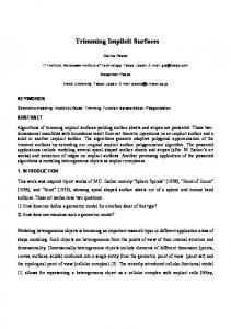
Given a set of n distinct constraint points {c1 , c2 , . . . , cn }, 1 cxk cyk c ∈ r since in this case δ(s1 , S) > r. A cell C2 “distant” from S satisfies f (s2 ) > ∆ and thus also satisfies δ(s2 , S) > ∆. C2 can be discarded provided that r < ∆. distance between s and S is also greater than ∆, since all points p which are at a distance smaller than ∆ to S necessarily satisfy |f (p)| < ∆. Thus, we may state |f (x)| > ∆ ⇒ δ(x, S) > ∆.

Function Straddle performs the rejection test (9). It returns true if C straddles the surface f (x) = 0 and false otherwise. Unit (leaf) cubes correspond to the maximum subdivision level maxlevel. These are passed to function MCcellPolygonize, which performs the cell triangulation process [18]. The rejection test on these cubes is implicitly performed by the Marching Cubes standard procedure, i.e., by examining the signs of the function at the cube’s corners. A crucial consideration when implementing this algorithm is to avoid reevaluating the implicit function at points already visited. For instance, the “if” clause in step 2 evaluates the function at the center of cube C; this value may later correspond to a cube corner in step 1.(a). Our implementation employs a cache of evaluated points so that f is computed only once for each space point.

(8) 5 Experiments

We may take advantage of this by making sure that the radius of C is never greater than ∆ since in this case |f (s)| > ∆ will necessarily imply δ(x, S) > r, meaning that the cell cannot intersect S (see Fig. 3). This assumption permits us to cover both cases (cell “near” or “far” from S) with a single simple rejection test: |f (s)| > r ⇒ C does not straddle S.

(9)

One last issue remains to be addressed: how is ∆ established? In practice, there is no need to compute a fixed value for ∆, but merely to ensure that it is large enough, i.e., that the largest cell radius used in the polygonization process is never greater than ∆. This is accomplished by using a sufficiently large ratio between d and w (see Fig. 4). Nonetheless, too large a ratio will have a detrimental effect on the algorithm performance. To see this, notice that in this case, f (x) will return too low an estimate for δ(x, S) in many cases, thus requiring many cells to be subdivided needlessly. We conducted several experiments (see Section 5) that indicate that d = 4w/3 is usually a large enough ratio without incurring in heavy performance penalties. The space sampling algorithm used in our implementation is summarized in the following pseudo-code: procedure SpaceSample(f , C, maxlevel, level) 1. If (level == maxlevel) then (a) Evaluate f at those corner points of C that were not yet evaluated; (b) MCcellPolygonize(C);

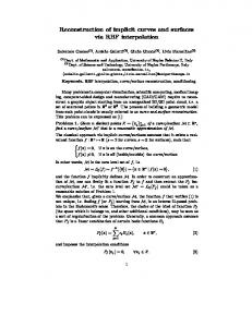
The experiments were performed on a PC equipped with an AMD-Duron processor running at 1.3 GHz and 256 MB of main memory. All models were simplified down to 800 vertices and placed inside a cubical space with (-1,-1,-1) and (1,1,1) as minimum and maximum points, respectively. In our implementation the cubical space is uniformly divided into a 3D grid of identical cubes whose size is s × s × s, where s is a power of two. We first conducted experiments aimed at finding “optimal” values for the maximum cell radius r and for the w/d ratio. For this purpose, we performed the polygonization of the “Stanford Bunny” data set using six values of w/d (0.2, 0.5, 0.667, 0.75, 0.8 and 0.83) and six values for r. Since we use an octree-like decomposition scheme, the six values of r correspond to the octant radii of consecutive √ √ refinement levels of the initial cubic space, i.e., 3/2, 3/4, and so forth. In Table 1 we observe the direct relation between different values of r and w/d . A small w/d ratio implies a large ∆ size, making it possible to use large initial sizes for r while still yielding a correct polygonization. However, large ∆’s have a detrimental effect on the algorithm performance. Figure 4 illustrates how the value of ∆ depends on the w/d ratio. Recall that ∆ denotes the “size” of the region where f can be used as a lower bound for the Euclidean distance. Next, we performed other experiments to test the efficiency of the algorithm on the polygonization of some reconstruction functions. See results in Figure 5 and on

w 1 = d 5 w 1 = d 2 w 2 = d 3 w 3 = d 4 w 4 = d 5 w 5 = d 6

√ 3 2

26.38% ok 12.36% ok 9.89% ok 9.01% ok 8.57% hole 8.29% hole

r=

√ 3 4


r=

√ 3 8


r=

√ 3 16


r=

√ 3 32

26.68% ok 13.26% ok 10.93% ok 10.10% ok 9.69% ok 9.42% hole

r=

√ 3 64

32.78% ok 21.94% ok 20.09% ok 19.44% ok 19.12% ok 18.90% ok

Table 1: This table shows results of the proposed algorithm in polygonizing the “Stanford Bunny” reconstruction function modeled with different values of w/d. d was set to 0.015 in all tests. The percentage values correspond to the total number of function evaluations required by the algorithm compared with the number of evaluations required by a standard Marching Cubes. A “hole” value means that resulting polygonization is incorrect, i.e., the algorithm rejected one or more cells straddling the surface. the left side of Table 2. All functions were built using 800-vertex polygonal meshes as input data and setting d = 0.015 and w/d = 3/4. The LU decomposition for solving the equations system took 42 s. in all experiments. The initial cube was initially subdivided in 128 × 128 × 128 cells. Finally, some experiments were performed to compare the proposed algorithm with the Bloomenthal’s continuation implementation [5]. In order to obtain a “fair” comparison, we had to modify Bloomenthal’s implementation so that its vertex computing function, which ordinarily uses binary subdivision, would employ linear interpolation instead. Moreover, the algorithm was configured to use cubical decomposition instead of the default tetrahedral decomposition. Also, a vertex of the polygonal mesh is used as the seed point. In both implementations, the cube sizes correspond to a 128 × 128 × 128 decomposition of the world space. The comparison results are shown in Table 2. The experiments indicate that the proposed technique tends to perform slightly faster than Bloomenthal’s implementation. As one might expect, the number of triangles for both methods are almost identical. The slight variation is due to the fact that the cubical decompositions are not the same, since the “seed” point used in Bloomenthal’s code determines the decomposition’s origin. The improved performance can be attributed to the smaller number of function evaluations performed by the proposed technique. We also tested the generated polygonizations for topological consistency with positive results. It should be noted, however, that the proposed technique is based on the Marching Cubes [18] algorithm and thus it inherits all its disad-

1,8 1,6 1,4 1,2 1 0,8 0,6 0,4 0,2 0 -1 ,0 0 -0 ,8 8 -0 ,7 6 -0 ,6 4 -0 ,5 2 -0 ,4 0 -0 ,2 8 -0 ,1 6 -0 ,0 4 0, 08 0, 20 0, 32 0, 44 0, 56 0, 68 0, 80 0, 92

r=

w/ d w/ d w/ d w/ d w/ d w/ d

= 1/ 5 = 1/ 2 = 2/3 = 3/ 4 = 4/5 = 5/ 6

d d d d d d

= 0.015 = 0.015 = 0.015 = 0.015 = 0.015 = 0.015

Figure 4: Plot of the various interpolating functions used in the experiments (see Table 1), evaluated on the line segment defined by (-1,-1,-1) and (1,1,1). vantages such as the creation of an excessively large number of triangles and the introduction of some ambiguities in lower resolutions. 6 Conclusions and future work We have presented a technique for the fast polygonization of variational implicit surfaces. This technique minimizes the number of the costly function evaluations using an hierarchical sampling of the space and thus permitting an efficient application of the Marching Cubes algorithm. The proposed technique can also be applied to the polygonization of other classes of implicit objects, as long as their generating functions behave as lower bounds for Euclidean distance metrics within a given neighborhood (see the discussion in Section 4.3). One important observation is that this condition is considerably weaker than the wellknown Lipschitz criteria exclusion [13]. Additionally, it should be possible to adapt the ideas presented in this paper to other visualization techniques. For instance, ray tracing of implicit surfaces could be efficiently performed by coupling the proposed voxel rejection criteria with standard octree-based speed-up techniques. To conclude, we would like to explore this technique in the context of FastRBF [7], adaptive polygonization scheme and the support of sharp features. Acknowledgments Many thanks are due to Dr. Marco Aurélio P. Cabral for his helpful insights. We are also grateful to CNPq for providing financial support for the first author.

Figure 5: Different models polygonized with the proposed technique. References [1] C. Bajaj, J. Blinn, J. Bloomenthal, M. Cani-Gascuel, A. Rockwood, B. Wyvill, and G. Wyvill. Introduction to Implicit Surfaces. Morgan Kaufmann Publishers, INC., San Francisco, California, 1997.

[7] J. C. Carr, R. K. Beatson, J. B. Cherrie, T. J. Mitchell, W. R. Fright, B. C. McCallum, and T. R. Evans. Reconstruction and representation of 3D objects with radial basis functions. In Proceedings of SIGGRAPH 2001, pages 67–76. ACM Press, 2001.

[2] R. K. Beatson, J. B. Cherrie, and D. L. Ragozin. Fast evaluation of radial basis functions: Methods for fourdimensional polyharmonic splines. SIAM J. Math. Anal., 32(6):1272–1310, 2001.

[8] J. C. Carr, R. K. Beatson, B. C. McCallum, W. R. Fright, T. J. McLennan, and T. J. Mitchell. Smooth surface reconstruction from noisy range data. In Proceedings of ACM Graphite 2003, pages 119–126. ACM Press, 2003.

[3] R. K. Beatson and W. A. Light. Fast evaluation of radial basis functions: Methods for two-dimensional polyharmonic splines. IMA Journal of Numerical Analysis, (17):343–372, 1997.

[9] B. Crespin. Dynamic triangulation of variational implicit surfaces using incremental delaunay tetrahedralization. In Proceedings of the 2002 IEEE Symposium on Volume Visualization and Graphics, pages 73–80, Piscataway, NJ, 28–29 2002. IEEE.

[4] J. Bloomenthal. Polygonization of implicit surfaces. Computer Aided Geometric Design, pages 341–335, November 1988. [5] J. Bloomenthal. An implicit surface polygonizer. Graphics Gems IV, pages 324–349, 1994. [6] M. D. Buhmann. Radial Basis Functions. Cambridge University Press, 2003.

[10] H. Q. Dinh, G. Turk, and G. Slabaugh. Reconstructing surfaces using anisotropic basis functions. In Proceedings of the Eighth International Conference On Computer Vision, pages 606–613, Los Alamitos, CA, July 2001. IEEE Computer Society. [11] H. Q. Dinh, G. Turk, and G. Slabaugh. Reconstructing surfaces by volumetric regularization using radial basis functions. In IEEE Transactions on Pattern Analy-

The proposed algorithm

Constraint

Model Bunny Horse Torus2 Hand Head Knot

Bloomenthal’s algorithm

points

Iso-surface

Evaluations

Triangles

Evaluations

Iso-surface

Evaluations

Triangles

(number)

extraction

(number)

(number)

(%)

extraction

(number)

(number)

1600 1600 1600 1599 1600 1600

58s 34s 27s 26s 53s 81s

193395 111560 90654 83202 176270 269701

81340 47028 33932 34660 71528 114704

9.01% 5.20% 4.22% 3.87% 8.21% 12.56%

75s 43s 31s 32s 65s 104s

244171 141128 102867 104085 214441 343725

81420 47088 34304 34720 71508 114592

Table 2: Comparison between the Bloomenthal’s continuation algorithm and the proposed technique. sis and Machine Intelligence, pages 1358–1371. IEEE Computer Society, October 2002. [12] X. Jim, H. Sun, and Q. Peng. Subdivision interpolating implicit surfaces. Computer Graphics, pages 763–772, October 2003. [13] D. Kalra and A. Barr. Guaranteed ray intersections with implicit surfaces. Computer Graphics, pages 297–306, July 1989.

[21] Y. Ohtake, A. Belyaev, M. Alexa, G. Turk, and H.P. Seidel. Multi-level partition of unity implicits. ACM Transactions on Graphics, 22(3):463–470, July 2003. [22] P. Reuter, I. Tobor, C. Schlick, and S. Dedieu. Pointbased modelling and rendering using radial basis functions. In Proceedings of ACM Graphite, pages 111–118, Held in Melbourne, Australia, 2003. ACM Press.

[14] O. Karpenko, J. F. Hughes, and R. Raskar. Free-form sketching with variational implicit surfaces. Computer Graphics Forum, September 2002.

[23] V. Savchenko, A. Pasko, O. Okunev, and T. Kunii. Function representation of solids reconstructed from scattered surface points and contours. Computer Graphics Forum, 14(4):181–188, 1995.

[15] N. Kojekine. Computer Graphics and Computer Aided Geometric Design by means of Compactly Supported Radial Basis Functions. PhD thesis, Tokyo Institute of Technology, 2003.

[24] I. Tobor, P. Reuter, and C. Schlick. Efficient reconstruction of large scattered geometric datasets using the partition of unity and radial basis functions. Journal of WSCG, 12(1-3):467–474, February 2004.

[16] H. Laga, R. Piperakis, H. Takahashi, and M. Nakajima. A radial basis function based approach for 3d object modeling and reconstruction. In IWAIT2003, pages 139–144, 2003.

[25] G. M. Treece, R. W. Prager, and A. H. Gee. Regularised marching tetrahedra: improved iso-surface extraction. Computers and Graphics, 23(4):583–598, 1999.

[17] S. K. Lodha and R. Franke. Scattered data techniques for surfaces. In G. Nielson H. Hagen and F. Post, editors, Proceedings of Dagstuhl Conference on Scientific Visualization, pages 182–222, DagstuhlGermany, June 1999. IEEE Computer Society Press.

[26] G. Turk and J. O’Brien. Variational implicit surfaces. Technical report, Georgia Institute of Technology, May 1999.

[18] W. Lorensen and H. Cline. Marching cubes: a high resolution 3d surface construction algorithm. Computer Graphics, 21(4):163–169, July 1987. [19] S. V. Matveyev. Approximation of isosurface in the marching cube: Ambiguity problem. In Proceedings IEEE Visualization, pages 288–292. IEEE Computer Society, October 1994. [20] B. S. Morse, T. S. Yoo, P. Rheingans, D. T. Chen, and K. R. Subramanian. Interpolating implicit surfaces from scattered surface data using compactly supported radial basis functions. In Shape Modeling International, pages 89–98, Genova, Italy, May 2001.

[27] G. Turk and J. O’Brien. Modelling with implicit surfaces that interpolate. ACM Transactions on Graphics, pages 855 – 873, October 2002. [28] L. Velho, J. Gomes, and L. H. Figueiredo. Implicit Objects in Computer Graphics. Springer Verlag, New York, 2002. [29] H. Wendland. Piecewise polynomial, positive definite and compactly supported radial basis functions of minimal degree. AICM, (4):389–396, 1995. [30] G. Yngve and G. Turk. Robust creation of implicit surfaces from polygonal meshes. In IEEE Transactions on Visualization and Computer Graphics, pages 346–359. IEEE, 2002.