Institute of Computer Science, University of Würzburg. Am Hubland, 97074 .... Therefore, it is necessary to describe the content of the environment in a computer.
University of Wu¨rzburg Institute of Computer Science Research Report Series
Fast Ray-Tracing for Field Strength Prediction in Cellular Mobile Network Planning K. Tutschku Report No. 134
K. Leibnitz January 1996
Institute of Computer Science, University of W¨ urzburg Am Hubland, 97074 W¨ urzburg, Germany Tel.: +49-931-8885513, Fax: +49-931-8884601 e-mail: {tutschku,leibnitz}@informatik.uni-wuerzburg.de
Abstract: In this paper we present a fast ray-tracing technique with scalable approximation accuracy for field strength prediction in cellular mobile network planning. Automatic network design methods, like the Adaptive Base Station Positioning Algorithm (ABPA), [2, 3], perform a huge number of field strength estimations and require therefore a fast and accurate approximation. However, common prediction techniques either give only rough estimations or are too complex for fast evaluation, cf. [7]. The proposed new ray-tracing technique obtains its speed-up by taking advantage of the topological information inherent in the used triangulation data structure of the investigated terrain. By that, it is possible to apply simple mathematics and algorithms to trace individual rays. The applicability of the fast ray-tracing technique is demonstrated for both a single transmitter scenario and in conjunction with ABPA. Keywords: mobile communication, network planning, base station location, field strength prediction, ray-tracing
1
Introduction
The fast and careful planning of modern cellular mobile communication networks is an essential criterion for their commercial success. With the application of fast design methods, a network operator can reduce the planning costs and shorten the time of putting the system to operation. Additionally, careful network planning can keep the investments into required hardware on a minimal level while obtaining a high quality of service. The planning procedures for present mobile communication systems try to obey these essentials, cf. [4], but fulfill the objectives only partially. For example, commercial available mobile planning tools like GRAND, [6], help the system engineer to evaluate the radio coverage but they do not give a hint where to place the transmitters. The engineer has to move them around in the virtual planning scenario of the tool until he finds a good configuration. Moreover, nowadays applied planning methods concentrate only on radio engineering aspects, like radio coverage and interference. They neglect the user behavior and the related teletraffic issues.
2
Integrated mobile planning
The shortcomings mentioned above lead to the need for an unsupervised and integrated design method. The approach is summarized in Figure 1. The core component is the Adaptive Base Station Positioning Algorithm (ABPA) and was first presented in [2]. The algorithm autonomously locates base stations in the investigated terrain. ABPA considers four different system engineering aspects: the radio wave propagation, the user behavior, the teletraffic allocation and the system architecture. So far, only the first two aspects are implemented and the latter two are in planning. The spatial behavior of mobile users is represented within ABPA by a distribution of discrete cluster points, cf. [3]. For obtaining an optimal mobile service supply the algorithm uses competing base stations which try to cover as many points as possible. The algorithm shifts around the transmitter in the virtual scenario until a considerable configuration is reached. The movement of the base station is conducted by a modified simulated annealing procedure. Since this is an iterative algorithm, it requires the evaluation of the radio coverage in each adaption step. However, the prediction methods used for cellular network design are either too complex and therefore computationally intensive [7] or not accurate enough for automatic planning Adaptive Base Station Positioning Algorithm
user behaviour
teletraffic allocation
radio wave propagation
system architecture
Abbildung 1: Integrated Network Planning Approach 2
[9]. Because of this fact, ABPA requires a fast and arbitrary accurate field strength prediction method, i.e. the engineer must be able to adjust the speed by choosing a certain accuracy.
3
Radio wave propagation models
The accuracy of the field strength prediction depends particularly on the applied radio wave propagation model. A lot of different propagation models have been proposed for various environments, like urban or rural terrain. An efficient algorithm for the prediction has to regard the specific features of these models. In this section, we will not provide physical formulae, but an overview of some important field strength prediction methods and their capability. For a more detailed description of these methods, the interested reader is conferred to [1, 7, 9]. Free Space Propagation assumes that no obstacle interferes the radio wave propagation. Therefore the field strength depends only on the distance between the transmitter and the receiver. The approximation can be computed rapidly from one equation, but it estimates the actual value field only very roughly. A more realistic propagation model was presented by Okumura [8]. It is essentially based on computing the free space path loss and then adding or subtracting correction factors to account for the different morphological features of urban and rural terrain as well as the antenna height. The model was made applicable by Hata, cf. [5]. He published empirical values for the correction factors. Since the Okumura/Hata model is an extension of the Free Space Propagation model, it is quite simple to compute, but limited in accuracy. Complex propagation models like the methods described by K¨ urner et al. [7] are based on ray-optical approaches. The wave interactions are modeled in detail and described by the uniform theory of diffraction and physical optics. This approach is very accurate but it requires considerable computational effort, since conventional ray-tracing is applied. To sum up, there are many field strength prediction methods with different complexity, but a method with arbitrary scalable speed and accuracy is not available yet.
4
Fast Ray-Tracing
The field strength prediction method which we consider is based on the capability of ray-tracing to model optical effects very accurately. Ray-tracing was introduced by Whitted, [10], as a technique for creating photo-realistic pictures. Since ray-tracing for image generation and ray-tracing for field strength prediction have the same core idea but differ essentially, we first explain the image generation method and thereafter the field strength prediction approach.
4.1
Ray-Tracing for photo-realistic image generation
To generate high-quality pictures, photo-realistic ray-tracers consider the sum of all details within the picture, such as surface textures, shadows, reflections, etc. 3
secondary ray (shadow ray)
object
light source
primary rays
secondary ray (reflected ray)
image plane
shadowed region
observer
Abbildung 2: Schematics of ray tracing
Therefore, it is necessary to describe the content of the environment in a computer processable format. Usually, this is achieved by specifying all objects as certain graphical primitives, e.g. rectangles, cubes or spheres. The image is generated with this information in the rendering step, see Figure 2. This processing step assumes an observer which is looking at the modeled scenery from behind the image plane. The plane or window is segmented by a regular grid where each segment corresponds to a pixel of the generated picture. A ray originating at the observer is cast through the center of each pixel and traced until its first intersection with an object. The pixel color is set to the ambient color of this object. The color of the object is determined by recursively tracing and emitting secondary rays until a certain recursion depth is reached. By using secondary rays, this method can simulate optical effects like shadows, reflection, and refraction. Unfortunately, optical ray-tracers are slow because the simulation of these effects requires high computational effort. Moreover, they generate only a two-dimensional picture of the visible objects of the three-dimensional scenery. However, for evaluating the radio coverage, the electric field strength on every surface element in the scenery has to be computed.
4.2
Ray-Tracing for field strength prediction
Ray-tracing for field strength prediction is based on the light house idea, see Figure 3. The ray-tracer emits radio beams from the transmitter in all directions and illuminates the scenery, i.e. the supplying area. At an intersection the appropriate physical laws for reflection, diffraction, and transmission of radio waves are applied. Because of this direct ray-tracing, often also referred to as ray-launching, the field strength is obtained on each surface element. Furthermore, this approach includes the possibility of modeling multipath propagation. However, this method is still very slow, due to the lack of knowledge about the structure of the scenery.
4.3
Fast Ray-Tracing
Our proposed fast ray-tracing technique is based on the ray-launching approach and obtains a considerable speed up by using a sophisticated three-dimensional digital terrain model. The terrain is composed of triangles that interpolate the surface
4
primary rays
secondary ray (reflected ray)
light source
secondary ray (diffracted ray)
sphere object
shadowed region
Abbildung 3: Ray-launching
between the equidistant altitude samples, see Figure 4. By exploiting the topographical information inherent in this data structure, the fast ray-tracing method avoids unnecessary intersection tests of the emitted ray with the triangles. The projection of the triangles from the three-dimensional terrain model onto a two-dimensional (x, y)-plane takes on regular shapes (compare Figure 4). This facilitates a favorable numbering with three ordinates (x, y, z), where x and y are the ordinates of usual two orthogonal axes of the projection plane and z is the index of the diagonals. In the (x, y)-projection an emitted beam traverses a sequence of adjacent triangles, see Figure 5. The points that lie on intersections of the projection of the ray and the projection of the triangle edges are called trajectory points. They are stored as a sorted list. Once the list is obtained, an intersection of a ray with a surface element can be detected by comparing the height values ∆i and ∆i+1 of two successive trajectory points i and i + 1, see Figure 6. The height ∆i of a trajectory
x
y
z
start traj 1 traj 2
y min traj 3 traj 4 traj 5
Tx
traj 6 traj 7
y
y max
traj 8
x z
traj 9
x min
end
x max
Abbildung 5: Trajectory points of a ray
Abbildung 4: Three-dimensional terrain model 5
∆ h i-2 ∆ h i-1
traj i-2
∆hi
3D triangle model c
∆ h i+1
traj i-1 traj i
traj i+1
2D projection
Abbildung 6: Calculation of a three-dimensional intersection point point i is the altitude of the ray at this point relative to the surface, marked by the arrows in Figure 6. A change of sign of these height values indicates an incident ray. Once a point of intersection is determined, the electric field strength on this surface element can be computed by modeling the proper physical effects [7]. The list of trajectory points can be obtained by applying Algorithm 1. The proAlgorithm 1 (Generate Trajectory) variables: xmin , xmax ymin , ymax line x, y, z nump , numq , numd p, q, d traj
range of x values range of y values traced ray loop variables index variables indexed lists of points resulting list of trajectory points
algorithm: 1 2 3 4 5 6 7 8 9 10 11 12 13 14 15 16 17 18 19 20
funct gen trajectory(start, end) ≡ begin xmin ← Ceil(start.x); xmax ← Floor(end.x); ymin ← Ceil(start.y); ymax ← Floor(end.y); line ← new line(start, end); for x ← xmin to xmax do pnump ← point on line(line, x); nump ← nump + 1; od for y ← ymin to ymax do qnumq ← point on line(line, y); numq ← numq + 1; od for z ← xmin + ymin to xmax + ymax do dnumd ← point on line(line, z); numd ← numd + 1; od traj ← merge lists(p, q, d) return traj. end
Algorithm 1: Generate Trajectory 6
radiated surface element ∆ step Tx
trajectory points
Abbildung 7: Fixed altitude angle stepwidth cedure Generate Trajectory intersects the projected ray with the parallels of the x-axis which have integer y-coordinates and stores the trajectory points. Then, the parallels of the y-axis and the z-axis are treated analogously. It is important to mention at this point, that intersections in a two-dimensional space are much easier to compute than in a three-dimensional environment. In Algorithm 1, point on line() calculates the point on the line for a certain integer x, y, or z coordinate. The function new line() creates a new ray from start to end. The procedure merge lists() consists of a merge-sort routine and combines the three lists of axes trajectory points. A major drawback of common ray-launching methods is the appropriate setting of the stepwidth for the altitude and the latitude angle. For example, if the altitude angle ∆ step was selected too large, not every surface element is reached. If this angle was too small, too many superfluous beams are emitted, see Figure 7. This problem disappears if rays are aimed at the midpoints between every two successive trajectory points, see Figure 8. The complete fast ray-tracing algorithm is shown in Algorithm 2. The algorithm directs trajectory lines with latitude angle ϕ and computes their trajectory points. Then, the algorithm emits rays to the midpoints between two trajectory points, cf. Figure 8. An intersection of this ray with a surface element will occur in any case. The functions collision() computes the exact intersection point on the surface element. At this location the field strength is evaluated by the function fsp(), which models the proper physical effects, cf. [7]. The predicted field strength value is stored for each the surface element. Additionally, the intersection point serves as a starting point for secondary rays. The new beam is generated by function radiated surface element
Tx
trajectory points
Abbildung 8: Variable altitude angle stepwidth 7
Algorithm 2 (Fast Ray Tracing Algorithm) variables: radius current maximum range of Tx dist Eucl. distance between Tx and sensors fs temp. variable for field strength calculation traj list of trajectory points c intersection point of ray with triangles ti triangle of three dimensional terrain model ∆ϕ, ϕ horizontal stepping and tracing angle algorithm: 1 2 3 4 5 6 7 8 9 10 11 12 13 14 15 16 17 18 19 20 21 22 23 24 25 26 27 28 29 30 31 32 33 34 35 36
proc fast ray tracing(Tx) ≡ begin radius ← max range(Tx); for all triangles ti do ti .field strength ← 0; od for ϕ := 0 to 2 · Π step ∆ϕ do targettraj ← (Tx) + (sin(ϕ), cos(ϕ), 0); traj ← gen trajectory(Tx, targettraj ); for i := 1 to ktrajk do targetdecl ← 12 · (trajj−1 + trajj ); if distance(Tx, targetdecl ) < radius then line ← new line(Tx, targetdecl ); ∆hold ← antenna height(Tx); for j := 1 to i do ∆hnew ← hray − htriangle ; j j if sign(∆hnew ) < 0 then c ← collision(trajj−1 , trajj ); fi ∆hold ← ∆hnew ; od dist ← distance(Tx, c); f s ← fsp(Tx, dist); ti ← find triangle(c); ti .field strength ← f s; create secondary ray(c); fi od od for all sensors si do ti ← find triangle(c); si .field strength ← ti .field strength; od. end
Algorithm 2: Fast Ray-Tracing create secondary ray() and is recursively traced until a given depth is reached. The function find triangle() relates the intersection point with its encompassing triangle. The function max range() limits the length of the trajectory to the 8
Abbildung 9: Supplying area of a single transmitter
Abbildung 10: Result of fast ray-tracing with ABPA
maximum receiving distance and the function distance() computes the distance between two points in the three-dimensional model.
5
Results for a single transmitter
We applied our fast ray-tracing method on real terrain data of an area northwest of W¨ urzburg, Germany. The extension of the area is 10km × 10km. Figure 9 shows the bird’s eye perspective of the supplying area for a single transmitter located in the center. Points marked by ’x’ represent cluster points (of the spatial user distribution, cf. section 2), which receive a field strength above a certain threshold. The points marked by ’+’ are cluster points where radio coverage is not given. The shape of the supplying area has the expected “lacunarity” and is corroborated by results from real measurements.
6
Applying Fast Ray-Tracing for locating multiple base stations
Figure 10 shows the final distribution of six base stations using ABPA in conjunction with fast ray-tracing. The transmitters are marked by the radio towers and the different supplying areas for the individual transmitters are tagged by various symbols. The result was obtained on a SUN SparcStation 20/612 in less than two hours. The final placement of the transmitter was plausible to human experts.
7
Conclusion
In this paper we presented a fast ray-tracing technique for field strength prediction. The proposed method obtains its speed-up by taking advantage of the topological information inherent in the used triangulation data structure. The appealing feature 9
is its scalability. By varying the triangle sizes, the stepwidth of the latitude angle, or the considered physical phenomena, it is possible to obtain the desired prediction accuracy or the intented speed. This fast ray-tracing methods permits the application of automatic cellular mobile network planning tools. Acknowledgment: The authors like to thank Prof. P. Tran-Gia for supporting their work.
References [1] J. B. Andersen, T. S. Rappaport, and S. Yoshida. Propagation messurements and models for wireless communications channels. IEEE Communications Magazine, 33(1):42–49, 1995. [2] T. Fritsch and S. Hanshans. An integrated approach to cellular mobile communication planning using traffic data prestructured by a self-organizing feature map. In Proceedings of the 1993 International Conference on Neural Networks, pages 822D–822I. IEEE, IEEE Service Center, M¨arz 28 – April 1 1993. [3] T. Fritsch, K. Tutschku, and K. Leibnitz. Field strength prediction by raytracing for adaptive base station positioning in mobile communication networks. In Proceedings of the 2nd ITG Conference on Mobile Communication ’95, Neu Ulm. VDE, Sep. 26 – Sep. 28 1995. [4] A. Gamst, E.-G. Zinn, R. Beck, and R. Simon. Cellular radio network planning. IEEE Aerospace and Electronic Systems Magazine, 1:8–11, Februar 1986. [5] M. Hata. Empirical formula for propagation loss in land mobile radio services. IEEE Transactions on Vehicular Technology, VT-29(3):317–325, 1980. [6] M. Kr¨ uger and R. Beck. Grand - Ein Programmsystem zur Funknetzplanung. Philips (PKI) - Technische Mitteilungen 2, 2:7–12, November 1990. [7] T. K¨ urner, D. Cichon, and W. Wiesbeck. Concepts and results for 3D digital terrain-base wave propagation models: an overview. IEEE Journal on Selected Areas in Communications, 11(7):1002–1012, September 1993. [8] Y. Okumura, E. Ohmori, T. Kawano, and K. Fukuda. Fieldstrength and its variability in VHF and UHF land mobile radio service. Review of the Electrical Communication Laboratory, 16(9-10):825–873, 1968. [9] D. Parsons. The Mobile Radio Propagation Channel. Pentech Press, London, 1992. [10] T. Whitted. An improved illumination model for shaded display. Communications of the ACM, 23(6):343–349, 1980.
10
Preprint-Reihe Institut fu ¨ r Informatik Universit¨at Wu ¨rzburg Verantwortlich: Die Vorst¨ande des Institutes f¨ ur Informatik. [90] U. Hertrampf. On Simple Closure Properties of #P. Oktober 1994. [91] H. Vollmer und K. W. Wagner. Recursion Theoretic Characterizations of Complexity Classes of Counting Functions. November 1994. [92] U. Hinsberger und R. Kolla. Optimal Technology Mapping for Single Output Cells. November 1994. [93] W. N¨oth und R. Kolla. Optimal Synthesis of Fanoutfree Functions. November 1994. [94] M. Mittler und R. M¨ uller. Sojourn Time Distribution of the Asymmetric M/M/1//N – System with LCFS-PR Service. November 1994. [95] M. Ritter. Performance Analysis of the Dual Cell Spacer in ATM Systems. November 1994. [96] M. Beaudry. Recognition of Nonregular Languages by Finite Groupoids. Dezember 1994. [97] O. Rose und M. Ritter. A New Approach for the Dimensioning of Policing Functions for MPEG-Video Sources in ATM-Systems. Januar 1995. [98] T. Dabs und J. Schoof. A Graphical User Interface For Genetic Algorithms. Februar 1995. [99] M. R. Frater und O. Rose. Cell Loss Analysis of Broadband Switching Systems Carrying VBR Video. Februar 1995. [100] U. Hertrampf, H. Vollmer und K. W. Wagner. On the Power of Number-Theoretic Operations with Respect to Counting. Januar 1995. [101] O. Rose. Statistical Properties of MPEG Video Traffic and their Impact on Traffic Modeling in ATM Systems. Februar 1995. [102] M. Mittler und R. M¨ uller. Moment Approximation in Product Form Queueing Networks. Februar 1995. [103] D. Rooß und K. W. Wagner. On the Power of Bio-Computers. Februar 1995. [104] N. Gerlich und M. Tangemann. Towards a Channel Allocation Scheme for SDMA-based Mobile Communication Systems. Februar 1995. [105] A. Sch¨omig und M. Kahnt. ∆Vergleich zweier Analysemethoden zur Leistungsbewertung von Kanban Systemen. Februar 1995. [106] M. Mittler, M. Purm und O. Gihr. Set Management: Synchronization of Prefabricated Parts before Assembly. M¨arz 1995. [107] A. Sch¨omig und M. Mittler. Autocorrelation of Cycle Times in Semiconductor Manufacturing Systems. M¨arz 1995. [108] A. Sch¨omig und M. Kahnt. Performance Modelling of Pull Manufacturing Systems with Batch Servers and Assembly-like Structure. M¨arz 1995. [109] M. Mittler, N. Gerlich und A. Sch¨omig. Reducing the Variance of Cycle Times in Semiconductor Manufacturing Systems. April 1995. [110] A. Sch¨omig und M. Kahnt. A note on the Application of Marie’s Method for Queueing Networks with Batch Servers. April 1995. [111] F. Puppe, M. Daniel und G. Seidel. ∆Qualifizierende Arbeitsgestaltung mit tutoriellen Expertensystemen f¨ ur technische Diagnoseaufgaben. April 1995. [112] G. Buntrock, und G. Niemann. Weak Growing Context-Sensitive Grammars. Mai 1995. [113] J. Garc´ıa and M. Ritter. Determination of Traffic Parameters for VPs Carrying DelaySensitive Traffic. Mai 1995.
11
[114] M. Ritter. Steady-State Analysis of the Rate-Based Congestion Control Mechanism for ABR Services in ATM Networks. Mai 1995. [115] H. Graefe. ∆Konzepte f¨ ur ein zuverl¨assiges Message-Passing-System auf der Basis von UDP. Mai 1995. [116] A. Sch¨omig und H. Rau. A Petri Net Approach for the Performance Analysis of Business Processes. Mai 1995. [117] K. Verbarg. Approximate Center Points in Dense Point Sets. Mai 1995. [118] K. Tutschku. Recurrent Multilayer Perceptrons for Identification and Control: The Road to Applications. Juni 1995. ¨ [119] U. Rhein-Desel. ∆Eine Ubersicht“ u ¨ber medizinische Informationssysteme: Krankenhaus” informationssysteme, Patientenaktensysteme und Kritiksysteme. Juli 1995. [120] O. Rose. Simple and Efficient Models for Variable Bit Rate MPEG Video Traffic. Juli 1995. [121] A. Sch¨omig. On Transfer Blocking and Minimal Blocking in Serial Manufacturing Systems — The Impact of Buffer Allocation. Juli 1995. [122] Th. Fritsch, K. Tutschku und K. Leibnitz. Field Strength Prediction by Ray-Tracing for Adaptive Base Station Positioning in Mobile Communication Networks. August 1995. [123] R. V. Book, H. Vollmer und K. W. Wagner. On Type-2 Probabilistic Quantifiers. August 1995. [124] M. Mittler, N. Gerlich, A. Sch¨omig. On Cycle Times and Interdeparture Times in Semiconductor Manufacturing. September 1995. [125] J. Wolff von Gudenberg. Hardware Support for Interval Arithmetic - Extended Version. Oktober 1995. [126] M. Mittler, T. Ono-Tesfaye, A. Sch¨omig. On the Approximation of Higher Moments in Open and Closed Fork/Join Primitives with Limited Buffers. November 1995. [127] M. Mittler, C. Kern. Discrete-Time Approximation of the Machine Repairman Model with Generally Distributed Failure, Repair, and Walking Times. November 1995. [128] N. Gerlich. A Toolkit of Octave Functions for Discrete-Time Analysis of Queuing Systems. Dezember 1995. [129] M. Ritter. Network Buffer Requirements of the Rate-Based Control Mechanism for ABR Services. Dezember 1995. [130] M. Wolfrath. Results on Fat Objects with a Low Intersection Proportion. Dezember 1995. [131] S. O. Krumke and J. Valenta. Finding Tree–2–Spanners. Dezember 1995. [132] U. Hafner. Asymmetric Coding in (m)-WFA Image Compression. Dezember 1995. [133] M. Ritter. Analysis of a Rate-Based Control Policy with Delayed Feedback and Variable Bandwidth Availability. January 1996. [134] K. Tutschku and K. Leibnitz. Fast Ray-Tracing for Field Strength Prediction in Cellular Mobile Network Planning. January 1996.
12