1 Walt Disney Animation Studios. 2 University of Utah. 3 Stanford University. 4 NVIDIA Corporation. Figure 1: Computing shadows using a prefiltered BVH is ...
Raytracing Prefiltered Occlusion for Aggregate Geometry Dylan Lacewell1,2 1
Brent Burley1
Walt Disney Animation Studios
2
Solomon Boulos3
University of Utah
3
Peter Shirley4,2
Stanford University
4
NVIDIA Corporation
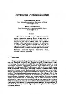
Figure 1: Computing shadows using a prefiltered BVH is more efficient than using an ordinary BVH. (a) Using an ordinary BVH with 4 shadow rays per shading point requires 112 seconds for shadow rays, and produces significant visible noise. (b) Using a prefiltered BVH with 9 shadow rays requires 74 seconds, and visible noise is decreased. (c) Reducing noise to a similar level with an ordinary BVH requires 25 shadow rays and 704 seconds (about 9.5× slower). All images use 5 × 5 samples per pixel. The scene consists of about 2M triangles, each of which is semi-opaque (α = 0.85) to shadow rays.
A BSTRACT We prefilter occlusion of aggregate geometry, e.g., foliage or hair, storing local occlusion as a directional opacity in each node of a bounding volume hierarchy (BVH). During intersection, we terminate rays early at BVH nodes based on ray differential, and composite the stored opacities. This makes intersection cost independent of geometric complexity for rays with large differentials, and simultaneously reduces the variance of occlusion estimates. These two algorithmic improvements result in significant performance gains for soft shadows and ambient occlusion. The prefiltered opacity data depends only on geometry, not lights, and can be computed in linear time based on assumptions about the statistics of aggregate geometry. 1 I NTRODUCTION Soft shadows and ambient occlusion are important tools for realistic shading in film production. However, these effects are expensive because they require integration of global visibility at each shading point. In a ray-based renderer, many shadow rays per shading point may be needed to accurately estimate visibility without noise artifacts. Variance is especially a problem with aggregate geometry, i.e., geometry consisting of a many small, disconnected parts, each of which may not be fully opaque. Examples frequently occurring in production include hair and foliage. In this paper we show how to reduce the cost of visibility queries for aggregate geometry by raytracing against a modified bounding volume hierarchy (BVH) in which we store a prefiltered opacity at each node, representing the combined visibility of all geometry contained in the node. Prefiltering requires a modest increase in the time to build or update a BVH; we demonstrate empirically that for
aggregate geometry, it suffices to use a prefiltering algorithm that is linear in the number of nodes in the BVH. Once built, a prefiltered BVH does not need to be updated unless geometry changes. During rendering, we terminate shadow rays at some level of the BVH, dependent on the differential [10] of each ray, and return the stored opacity at the node. The combined opacity of the ray is computed by compositing the opacities of one or more nodes that the ray intersects, in any order. This early termination eliminates many ray-triangle intersections, and makes intersection cost independent of geometric complexity for rays with large enough differentials. In addition, prefiltering also reduces the variance of occlusion estimates on aggregate geometry, which in turn reduces noise artifacts for a given number of shadow rays. Both benefits are demonstrated in Figure 1. The original contributions in this paper are as follows: • We prefilter directional opacity; previous work focused on prefiltering color. • We present a simple linear-time opacity prefiltering algorithm based on assumptions about the statistics of aggregate geometry. • We store prefiltered data in a BVH, a popular sparse acceleration structure that can be updated in linear time for many types of dynamic scenes [25]. • We show empirically that prefiltering reduces the cost of computing soft shadows and ambient occlusion. A note about terminology: we use opacity or occlusion interchangeably to mean the percentage of light that is blocked between two points, and visibility as the complement of occlusion. 2 BACKGROUND We discuss only the most relevant work on visibility queries. We refer the reader to the survey of shadow algorithms by Woo et al. [29],
or the more recent survey of real-time algorithms by Hasenfratz et al. [7]. 2.1
Raytracing
Distribution raytracing [5] is a general rendering method for many global illumination effects, including shadows, and can be used with prefiltered scenes. Mitchell [15] provided insights into how the convergence of raytracing depends on the variance of the scene. Variants of ray tracing such as packets [26], cone tracing [1], beam tracing [8, 17], and the shadow volumes method of Laine et al. [13] exploit geometry coherence to speed up intersection or reduce variance; these methods are less effective for aggregate geometry with small pieces but would benefit from prefiltered geometry. Precomputed radiance transfer [24] stores a raytraced reference solution at each shading point, in a basis that allows environment lighting at an infinite distance to be updated dynamically. True area lights at a close distance are not easily accounted for. 2.2
Point Hierarchies
Many previous methods have estimated scene visibility using multiresolution hierarchies of points, spheres, or other primitives. Very few point-based methods prefilter opacity, and most are demonstrated on solid, connected geometry. Bunnell [3] uses a hierarchy of disks, where disk sizes and positions are averaged, but changes in opacity due to empty space are ignored. Multiple rendering passes are required to correctly handle overlapping occluders. Pixar’s Photorealistic Renderman (PRMan) [18] appears to use a similar method. Wand [27] renders soft shadows by cone tracing a point hierarchy, but does not handle opacity changes due to empty space, and observes that shadows for foliage are overly dark. Ren et al. [20] approximate geometry with sets of opaque spheres, and splat spheres using a spherical harmonic technique that corrects for occluder overlap in a single pass. No solution for opacity filtering is given. Kontkanen and Lane [12] compute ambient occlusion by splatting opaque objects using precomputed visibility fields. Kautz et al. [11] rasterize scene visibility into a small buffer at each shading point; this is conceptually similar to point-based occlusion, but mesh simplification is used rather than a point hierarchy. Mesh simplification does not work well for aggregate geometry. A number of previous methods rasterize or raytrace very large point sets, mostly for direct viewing [9, 22, 31]. The prefiltering method employed is almost always averaging of point attributes, without regard to accumulated directional opacity. Neyret [16] does more precise prefiltering on an octree: surface color and normals are modeled with ellipsoids, and filtered in a relatively principled way. Opacity is averaged, not composited, and only shadows from point lights are demonstrated. Stochastic simplification [4] specifically targets aggregate geometry, and prefilters by removing primitives randomly and changing the sizes and colors of remaining primitives to maintain statistical properties. This method could be used for direct rendering while using our method for shadows. 2.3
Shadow Maps
Shadow maps are a common method for rendering shadows in games and film production. Traditional shadow maps precompute visibility in a scene for a frustum of rays originating at the light origin; no other visibility queries are supported. Deep Shadow Maps [14] and other multi-layer data structures [30] store a continuous opacity function along each ray, which is needed for aggregate geometry. Shadow maps support constant-time queries, and are built by rendering the scene in a separate pass, which is fast for scenes of moderate complexity. However, shadow maps are less general than raytraced visibility. Occlusion from small area lights can be
approximated with a single shadow map, but occlusion from large and/or non-planar lights cannot. Although it is possible to represent area lights using many shadow maps [21], computation time grows linearly with number of lights. The cost of building a shadow map is high for very complex scenes. The resolution of shadow maps in production may be as much as 16K × 16K, to ensure there are no aliasing artifacts; at our studio we have occasionally even seen shadow map generation take longer than final rendering. Separate maps are needed for every light in a scene, and these maps must be recomputed when either geometry or lights change. In contrast, our prefiltering method can reuse the same precomputed data for any configuration of lights, and for all instances of a given object. 2.4 Other work Probably the most common use of prefiltering is for mipmapping 2D surface color [28]. However, thinking only of this example can be misleading: averaging is (approximately) correct for diffuse surface color, but not for normals or 3D opacity. Mesh simplification, e.g., using a quadric error metric [6], can be viewed as prefiltering, but does not explicitly preserve opacity, and does not work well for aggregate geometry. 3 P REFILTERING O CCLUSION Recall that our goal is to store prefiltered opacity in a BVH and use this information to speed up visibility queries during rendering. In this section we motivate this goal using Monte Carlo rendering theory, then give the details of how we prefilter a BVH, and how we intersect rays with a BVH using solid angle comparisons. 3.1 Theory The irradiance at a surface point p with normal N is given by the following integral: Z
H(p, N) = S
V (p, ω)L f (p, ω)(ω · N)dω
where V (p, ω) is a visibility function that returns a value in [0, 1], L f (p, ω) is the incident radiance as seen by p in direction ω, and S is a region of the unit hemisphere with solid angle Ω(S). Ambient occlusion makes the approximation that L f = 1 and also adds a distance term to visibility. Direct illumination for soft shadows can also be rewritten as a sum over many lights instead of as an integral over the hemisphere. Traditional Monte Carlo rendering samples the area source uniformly in area with M samples and estimates the integral with the following sum: H0 =
A M cos θ cos θ 0 ∑ V (p, p0i )Le (p0i , p − p0i ) kp − p0 k2 M i=1 i
where A is the area of the light source, p0i is a point chosen on the light source, having normal N 0 , and the angles θ and θ 0 are between the light direction vector p − p0i and the normals N and N 0 respectively. Le is the surface radiance of the light, and is often constant. Visibility is evaluated by casting a shadow ray between points p and p0i . If instead the luminaire can be sampled directly according to the projected solid angle for the point p (see Shirley et al. [23] for examples where this is possible) the sum above can be rewritten as: H0 =
1 M ∑ V (p, ωi )L f (p, ωi )(ωi · N) M i=1
where V (p, ωi ) and L f (p, ωi ) are visibility and radiance samples computed by shooting a single shadow ray, with origin p and direction ωi . A single point sample is an estimate of irradiance over a small region Sr (ωi ) of the hemisphere having solid angle Ω/M.
Algorithm 1 occlusion(node, ray, t0 , t1 ) 1: // Exit early if ray misses bounding box. 2: hitInterval = node.getBound().rayIntersect(ray) 3: if hitInterval.clip(t0, t1).isEmpty() then 4: return 0.0 5: end if Figure 2: A shadow ray has a virtual cone defined by solid angle. We terminate the ray at (shaded) BVH nodes that fit within its cone, and return the composited prefiltered opacities of the two nodes. Nodes which do not intersect the ray are ignored, unlike with cone tracing. In either case, the rate at which the sum H 0 converges to the integral H is largely dependent upon the variance of V (p, ω), since Le is usually constant over the luminaire, and the cosine terms vary slowly. For scenes containing hair or vegetation, V may have very high variance, but a noisy estimate of H is not acceptable for production rendering. We can eliminate much of the variance by prefiltering V and replacing it with a similar function, V , that varies more slowly: V (p, ωi ) =
1 Ω(Sr )
Z
V (p, ω)dω Sr
For efficiency, we compute V before rendering, and store its approximate value for many possible regions of integration. Precomputed values of V can then be fetched and interpolated quickly during rendering. This is the motivation for storing opacity in BVH nodes: the opacity α of a node is the approximate value of 1 − V for the geometry within the node. 3.2 Ray Intersection using Solid Angles In our modified intersection scheme, each ray has an associated virtual cone defined by solid angle, Ωr = Ω(Sr ) and ray length. A virtual cone is a simple isotropic form of ray differential [10]. When intersecting each ray with the BVH, we compare the solid angle of the ray to the projected solid angle of the box, Ωb , and stop descending when Ωr /Ωb > T , where T is a user-defined threshold. Note that this is not the same as cone tracing; we are simply associating a solid angle with each ray but not performing exact intersection with a cone. For simplicity, instead of Ωb we use the projected solid angle of the bounding sphere of the box, Ωs = πR2 /|C − p|2 , where C is the box center and R is the radius. An intersection is diagrammed in Figure 2. Pseudo-code for a recursive ray-BVH intersection is shown in Algorithm 1; for clarity we assume that both child nodes exist and omit checking for null pointers, and also assume the existence of a triangleOcclusion function which returns 1 if a given ray and triangle intersect and 0 otherwise. When terminating, a ray-box intersection returns the approximate, pre-integrated opacity of the box, as viewed from the ray direction. We make the assumption that orthographic projection suffices, so that the opacity of the box depends only on viewing direction, ω, and not viewing position, p. This assumption has proven valid in practice, and becomes increasingly accurate as the number of rays increase and their solid angles decrease. The final opacity of a shadow ray is computed by compositing the opacities of every interior node or leaf triangle at which the ray terminates. Nodes can be intersected in any order. This algorithm avoids all ray-box and ray-triangle intersections below the termination depth in the BVH. However, since by design prefiltered nodes are rarely opaque, it is likely that the ray intersects multiple interior nodes. We show in the results section that this trade off is beneficial for complex geometry and semi-opaque geometry.
6: 7: 8: 9: 10: 11: 12: 13: 14: 15: 16: 17: 18: 19: 20: 21: 22: 23: 24: 25: 26: 27: 28: 29: 30: 31: 32: 33: 34: 35: 36: 37: 38: 39: 40:
3.3
// Descend immediately if node is below correlation height. if node.height()