Fast Rule Identification and Neighbourhood Selection for ... - CiteSeerX

IEEE TRANSACTIONS ON SYSTEMS, MAN, AND CYBERNETICS PART B: CYBERNETICS, VOL. XX, NO. XX, OCTOBER 2010

1

Fast Rule Identification and Neighbourhood Selection for Cellular Automata Xianfang Sun, Paul L. Rosin, Ralph R. Martin

Abstract—Cellular automata (CA) with given evolution rules have been widely investigated, but the inverse problem of extracting CA rules from observed data is less studied. Current CA rule extraction approaches are both time-consuming, and inefficient when selecting neighbourhoods. We give a novel approach to identifying CA rules from observed data, and selecting CA neighbourhoods based on the identified CA model. Our identification algorithm uses a model linear in its parameters, and gives a unified framework for representing the identification problem for both deterministic and probabilistic cellular automata. Parameters are estimated based on a minimum-variance criterion. An incremental procedure is applied during CA identification to select an initial coarse neighbourhood. Redundant cells in the neighbourhood are then removed based on parameter estimates, and the neighbourhood size is determined using a Bayesian information criterion. Experimental results show the effectiveness of our algorithm, and that it outperforms other leading CA identification algorithms. Index Terms—Cellular automata, rule identification, neighbourhood selection.

I. I NTRODUCTION ELLULAR Automata (CA) are a class of spatially and temporally discrete mathematical systems characterized by local interaction and synchronous dynamical evolution [1]. CAs were proposed by Von Neumann and Ulam in the early 1950s [2] as models for self-replicating systems. Since then, CA properties have been widely investigated, and CAs have been applied to simulating and studying phenomena in complex systems [3], [4], in such diverse fields as pattern recognition, physical, biological, and social systems [5]. Currently, much research still focuses on analysing CAs with known or designed evolution rules and using them in particular applications such as urban modelling and image processing. However, in many applications, formulating suitable rules is not easy [6], [7], [8]: often, only the desired initial and final patterns, or the evolution processes, are known. To be able to apply a CA, underlying rules for the CA must be identified. Some research already exists on this topic, but various fundamental problems remain. In particular, rule identification is typically computationally expensive, and neighbourhood selection is also a tricky problem. CA rule identification goes back to Packard et al. [9], [10], where genetic algorithms (GAs) were used to extract CA rules. Many later works also use GAs, or more general evolutionary algorithms, as a tool to learn CA rules [11], [12],

C

Manuscript received XXXX The authors are with the School of Computer Science & Informatics, Cardiff University, 5 The Parade, Roath, Cardiff CF24 3AA, UK. E-mail: {xianfang.sun, paul.rosin, ralph.martin}@cs.cardiff.ac.uk.

[13]. However, such approaches are time-consuming, while if the population size and number of generations are insufficient, suboptimal results are produced. Other parameters also need to be chosen carefully. Recently, Rosin [8], [14] considered training CAs for image processing, using the deterministic sequential floating forward search method to select rules. This approach is faster than those based on evolutionary algorithms, but is still slow. Adamatzky [15], [16] proposed several approaches to extracting rules for different classes of CA without resorting to evolutionary algorithms. For deterministic cellular automata (DCA), he starts with a minimal neighbourhood comprising only a central cell, collects data associated with the neighbourhood, and then extracts rules directly from that data. If contradictory rules occur, the radius of the neighbourhood is increased, data are re-collected, and rules are re-extracted from the enlarged data. This is repeated until no contradictory rules are generated, or a maximum neighbourhood size is reached. For probabilistic cellular automata (PCA), a similar procedure is used, but with different output and stopping criteria: it stops when a sequence of outputs, which are state transition probability matrices, has converged as a Cauchy sequence, or a maximum neighbourhood size or runtime has been reached. Calculation is fast, but the final neighbourhood may contain redundant neighbours if the target neighbourhood is not symmetric about the central cell. Maeda et al. [17] used the same approach as Adamatzky [16] to extract rules, but with a heuristic procedure to remove redundant cells. They further used a decision tree and genetic programming to simplify the CA state transition rules. Unfortunately, their technique can only deal with DCA. Also, their redundant cell removing procedure requires costly re-collection of data and re-identification each time a neighbourhood cell is removed. Using parameter estimation methods from the field of system identification, Billings et al. have developed a series of CA identification algorithms [18]. While their early work also used GAs for CA rule extraction [12], [19], [20], one of their main contributions was to introduce polynomial models to represent CA rules and an orthogonal least-squares (OLS) algorithm to identify these models [19], [21], [22]. This makes CA rule extraction a linear parameter estimation problem, allowing faster solutions. Many new identification algorithms [23], [24], [25], [26], [27], [28], [29] can also be used to solve the estimation problem. Other contributions have been made for neighbourhood selection, either as a by-product of the OLS algorithm [19], [21], or based on statistical approaches [30] or mutual information [31]. CA identification algorithms for binary CA have also been extended to n-state CA and spatio-


temporal systems [32], [33]. The main drawback of these algorithms is their inefficiency for CAs with large neighbourhoods. Overall, speed is the major problem for most current CA identification algorithms, coupled with inefficient neighbourhood selection. We show how to overcome these problems. Our main contributions are (i) a fast identification algorithm for extracting CA rules from input data, (ii) a simple neighbourhood reduction method which can remove redundant neighbours, or optionally remove non-redundant but insignificant neighbours, and (iii) use of the Bayesian information criterion (BIC) to determine optimal neighbourhood size. Our algorithms are faster than prior algorithms, while our neighbourhood selection method produces appropriate results as demonstrated experimentally. In the following, Section II introduces CAs, and presents a unified identification model for both DCA and PCA. Section III describes a CA rule identification method based on minimum-variance parameter estimation. Algorithms are provided for cases with and without given neighbourhoods. Section IV gives a method for deleting redundant cells from a neighbourhood based on parameter estimation, and a neighbourhood selection method based on the BIC. Section V compares the time and space complexity of our algorithm with others, while Section VI experimentally demonstrates the effectiveness of our algorithms and validates the complexity analysis and comparison. Section VII concludes the paper.

which are enumerated as: if Ni (t) = {0, . . . , 0}, then xi (t + 1) = f0 ; if Ni (t) = {0, . . . , 1}, then xi (t + 1) = f1 ; .. . if Ni (t) = {m − 1, . . . , m − 1}, then xi (t + 1) = fmn −1 . The left-hand-side of each rule is used to match the pattern of neighbourhood state values, while the right-hand-side gives the corresponding new state. Each fj can be any value in S, and is chosen according to the desired CA behaviour. If all rules are deterministic, i.e. F is deterministic, then the CA is a deterministic cellular automaton (DCA). In realworld systems, disturbances exist, and can cause uncertainty in the transition rules. Thus some of the fj take values statistically distributed in S. Such a CA is called a probabilistic cellular automaton (PCA). Normally, the rules of a PCA are represented by fj = {pj0 , . . . , pj(m−1) }, where pjk is the probability that the cell moves to state value k when its neighbourhood has the pattern j. Adamatzky [15] has provided algorithms for identifying {pjk }. However, in many cases, it is required to identify deterministic CA rules from data corrupted by noise, even though the CA behaves as a PCA. An alternative way to express the rules of a PCA is to decompose fj into a deterministic part and a statistical noise term [20], giving xi (t + 1) = f (Ni (t)) + (Ni (t)),

II. C ELLULAR AUTOMATA AND I DENTIFICATION This section briefly introduces cellular automata (CA) and their identification. Basic concepts and notation used in this paper are presented. For further background, see [1] and [4].

2

(2)

where f (Ni (t)) is a deterministic term and (Ni (t)) is a noise term. The identification problem considered in this paper uses the formulation in Eqn. (2). B. Identification Problem

A. Cellular Automata A CA can be described by a quadruple hC, S, N, f i comprising a d-dimensional cellular space C, an m-value state space S, an n-cell neighbourhood N , and a cell-state transition function f : S n → S. The cells in C typically form a regular, usually orthogonal, lattice, although 2D hexagonal lattices are also encountered. Recently, irregular grid structures have also been used to connect cells [34]. The cells have states normally represented by the numbers {0, . . . , m − 1}. The neighbourhood N of a cell consists of n cells which are usually spatially close to the cell; sometimes, the cell itself is included in this neighbourhood. The cell-state transition function f determines the state of a cell at the next time step according to the current states of the cells in its neighbourhood. All cells change states synchronously at each time step, and the cell states evolve the same function f at each time step. Let xi (t) be the state value of cell ci at time step t, and Ni (t) = {xli (t) : cli ∈ Ni , (l = 1, . . . , n)} be the state values of the cells in ci ’s neighbourhood Ni at time t. The state value of ci at time t + 1 is given by xi (t + 1) = f (Ni (t)).

(1)

Since the state set S is limited to m values, the cell-state transition function f can be represented by a set of (mn ) rules,

We now consider the problem of CA identification. Here, we only consider CAs with binary states, so m = 2. The spatial dimension of a CA does not actually matter, because in the identification of CA rules, only the state values are used for each state in their neighbourhood—the precise locations of the neighbouring cells are not taken into account. For a DCA, the state transition function can be represented as n 2X −1 xi (t + 1) = θj Qji (t), (3) j=0

where Qji (t) is the value of j th neighbourhood pattern defined by n Y Qji (t) = blj (xli (t)), (4) l=1

blj

and is defined as the coefficient of 2l−1 in j when j is written as a binary number. Note that for any state combination of {xli (t), (l = 1, . . . , n)}, only one pattern of {Qji (t), j = 0, . . . , 2n − 1} has value 1, and all others have value 0. θj is either 0 or 1, and θj = 0 represents the CA rule that when the neighbourhood state combination is pattern Qji (t), xi (t + 1) takes value 0, while θj = 1 means that xi (t + 1) takes value 1.


The identification problem for DCA is to determine the parameters {θj }, such that all collected data pairs {(xi (t + 1), Ni (t))} are consistent with Eqn. (3). In principle, we need at least 2n collected data pairs in order to identify all the 2n parameters corresponding to the 2n CA rules. However, in practice, some neighbourhood patterns may never happen, so less than 2n parameters need to be identified, and fewer than 2n data pairs may be available. Following Eqn. (2), the analogue of Eqn. (3) for a PCA is xi (t + 1) =

n 2X −1

θj Qji (t) + (Ni (t)).

(5)

j=0

The identification problem for PCA is then to estimate the parameters {θj }, such thatn the variance of the noise term P2 −1 (Ni (t)) = xi (t + 1) − j=0 θj Qji (t) is minimised. Because DCA is a special case of PCA, we henceforth only study Eqn. (5). Mathematically, the identification problem can be formulated as   n 2X −1 {θˆj } = arg min variance xi (t + 1) − θj Qji (t) , (6) j=0

if we assume that the neighbourhood is known in advance. If no a priori neighbourhood is known, a selection approach must be used to determine a suitable neighbourhood. Our approach to finding an optimal neighbourhood and CA parameters (rules) is (i) to use an incremental neighbourhood algorithm to select an initial coarse neighbourhood and simultaneously identify the parameters, (ii) to remove redundant neighbours from this initial neighbourhood, and (iii) to remove insignificant neighbours from the neighbourhood based on a Bayesian information criterion (BIC). III. RULE I DENTIFICATION We now consider estimating the CA parameters {θj } from collected data pairs {(xi (t + 1), Ni (t))}. A parameter estimation algorithm for a CA with a predetermined neighbourhood is first introduced, and generalised to an incremental algorithm when the neighbourhood is not known. A. Rule Identification with Known Neighbourhood We first consider CA rule identification with known neighbourhood. To solve Eqn. (6), we use the collected data pairs {(xi (t + 1), Ni (t))} to estimate the variance. This gives  2 n T X C 2X −1 X 1 xi (t + 1) − θj Qji (t) , {θˆj } = arg min T C t=1 i=1 j=0 (7) where T is the number of time steps, C is the number of cells, and θˆj is the optimal estimate of parameter θj . For notational simplicity, we combine the two summations into one with K = T C terms, and use yk and Qjk to represent xi (t+1) and Qji (t), respectively. We can thus rewrite Eqn. (7) as  2 n K 2X −1 X 1 yk − {θˆj } = arg min θj Qjk  . (8) K j=0 k=1

3

Now, θj , yk , and Qjk can only be 0 or 1, and 02 = 0, 12 = 1. Furthermore, Qik Qjk = 0 for i 6= j, so the right-hand-side of Eqn. (8) leads to P2n −1 j j 2 PK 1 σ ˆ 2 (n) = K j=0 θ Qk k=1 yk − (9) PK P2n −1 j j 1 = K k=1 yk − j=0 θ r , where σ ˆ 2 (n) is the variance estimate when the neighbourhood size is n, and rj is the contribution of the θj -related pattern to the reduction of the variance: ! K K X X 1 j j j r = 2 yk Qk − Qk . (10) K k=1

k=1

Writing y¯k to denote logical NOT of yk , and using yk +¯ yk = 1, this can be expressed as ! K K X X 1 j j yk Qk − y¯k Qk . (11) rj = K k=1

k=1

The first sum is the number of occurrences when the j th neighbourhood pattern appears (Qjk = 1) with yk = 1, and the second is the number with yk = 0 in all K data pairs. Eqn. (9) shows that minimising σ ˆ 2 (n) leads to an optimal j ˆ θ value of:   1, if rj > 0, j ˆ 0, if rj < 0, (12) θ =  u, if rj = 0, where u can be either 1 or 0: as rj = 0, it does matter whether θˆj is 1 or 0, because the θj -related pattern makes no contribution to the reduction of variance. Eqn. (11) shows that rj = 0 implies that: either the pattern Qjk never appears, or it appears as often with yk = 1 as with yk = 0 over all K data pairs. Although we could simply set u = 0, we choose not to fix it yet, as we can make good use of this freedom in neighbourhood selection. Afterwards, we can then set u = 0 to simplify rule description. B. Rule Identification with Incremental Neighbourhoods The above works if the correct neighbourhood is known, or an a priori neighbourhood is set. Otherwise, typically, a large enough initial neighbourhood is chosen to guarantee that the correct neighbourhood is included within it. After identifying the CA rules, the neighbourhood is reduced using some neighbourhood selection algorithm. However, too large an initial neighbourhood will result in excessive calculation. To avoid this problem, we use an approach similar to that in [15] to incrementally build the neighbourhood. Algorithm 1 describes our incremental algorithm, but we first explain the basic idea behind it. To begin with, we set a tolerance σT2 for the variance estimate σ ˆ 2 (n). The tolerance can be considered as the maximum rate at which the identified CA rules may produce results different from the observed ones. For a DCA, σT2 should be set to 0, while for a PCA, it should be set according to the noise level. If the noise level is unknown, a very small value should be used, to ensure that the correct neighbourhood is included in the selected neighbours.


Algorithm 1 Incremental Neighbourhood Algorithm Input: σT2 and {yk , xn k } (n = 1, . . . , nmax ; k = 1, . . . , K) j Output: {θˆ(n) ,σ ˆ 2 (n)} (n ≤ nmax ; j = 0, . . . , 2n − 1) Initialisation: PK σ ˆ 2 (n) = k=1 yk (n = 0, . . . , nmax ) Lk = yk (k = 1, . . . , K) n=0 while n < nmax and σ ˆ 2 (n) > KσT2 do n=n+1 rj0 = 0 (j = 0, . . . , 2n+1 − 1) for all k do Lk = Lk + 2n xn k 0 0 rL = rL +1 k k end for for j = 0 to 2n − 1 do 0 0 rj = r2j+1 − r2j j if r > 0 then θˆj = 1 (n)

σ ˆ 2 (n) = σ ˆ 2 (n) − rj j else if r < 0 then j θˆ(n) =0 else j θˆ(n) = u {Use any value other than 0 or 1 to represent u as a variable.} end if end for σ ˆ 2 (n) = σ ˆ 2 (n)/K end while

Using a small σT2 will result in low consistency between the observed data and the CA rules acting on a small neighbourhood, so to obtain high consistency between the data and CA rules, a larger neighbourhood is often required, increaseing the computational cost. More consideration is given to the selection of σT2 in Section VI-A. The incremental approach starts from a neighbourhood of size n = 1, and estimates the parameters and variance using the algorithm described in Section III-A. It adds one neighbour on each iteration until σ ˆ 2 (n) ≤ σT2 or we reach a stipulated maximum neighbourhood size n = nmax . Usually, the central cell ci is selected first, and when a new cell should be added to the neighbourhood, the cell closest to ci but outside the neighbourhood is selected. If this does not result in a unique choice, any can be used. j We now explain Algorithm 1. We denote by θ(n) the j th j parameter, yk the k th evolved state value, Q(n)k the k th value of the j th neighbourhood pattern for the neighbourhood of size n, xlk the k th state value of the lth neighbour. Initially, n = 1, and we set Q0(1)k = x ¯1k , and Q1(1)k = x1k . 0 1 θ(1) and θ(1) are calculated using Eqn. (12), while σ ˆ 2 (1) is j calculated using Eqn. (9) and r is calculated from Eqn. (11). When a new neighbour is added, the number of neighbourhood patterns is doubled from 2n to 2n+1 . As a result, σ ˆ 2 (n+ j 1) and θ(n+1) must be recomputed. The simplest approach is to recompute them ab initio from Equations (9), (11), and (12). While such an approach is taken by [15], this is inefficient. Instead, we use a recursive approach to calculate the parameter and variance estimates.

4 n−1

¯nk , and Qj+2 = Qj(n−1)k xnk Define Qj(n)k = Qj(n−1)k x (n)k j for j = 0, . . . , 2n−1 − 1. Clearly, Q(n)k = 1 only if j=

n X

xlk 2l−1 .

(13)

l=1

The algorithm uses a label Lk for each data pair to code its neighbourhood pattern and yk state, calculated by Lk = yk + 2j with j being defined by Eqn. (13). Note that Lk = 2j and Lk = 2j + 1 imply y¯k Qj(n)k = 1 and yk Qj(n)k = 1, 0 0 respectively. The numbers of occurrences, r2j and r2j+1 , of Lk = 2j and Lk = 2j+1 are used in Algorithm 1 as equivalent to the numbers of occurrences of y¯k Qj(n)k = 1 and yk Qj(n)k = 1, when using Eqn. (11) to calculate rj . Substituting Eqn. (13) into Lk and decomposing, we get Lk = (yk +

n−1 X

2l xlk ) + 2n xnk ,

(14)

l=1

which provides a basis for recursively calculating Lk . Algorithm 1 uses this recursively with for increasing neighbourhood size n. This allows us to find Lk for all neighbourhoods of sizes 1 to n using the same amount of computation as for just the single neighbourhood size n. IV. N EIGHBOURHOOD S ELECTION Algorithm 1 determines a large initial neighbourhood and CA parameter values. Typically, this neighbourhood contains some redundant neighbours, which can be removed from the neighbourhood without changing the CA behaviour. Further neighbours, which are not redundant but have very small effect on the CA behaviour, may also be removed to make the model parsimonious. We next discuss approaches for removing neighbours from the neighbourhood (Section IV-A) and optimal neighbourhood selection (Section IV-B). A. Neighbourhood Reduction We first consider how to eliminate redundant neighbours, then discuss how to remove non-redundant neighbours. Let j be an integer having 1 as its λth bit in its binary expression, and let jλ¯ have the same binary expression as j except that its λth bit is 0. From the definition of neighbourhood pattern in Eqn. (4), we get the merged pattern Y j Qji m (t) = Qji (t) + Qi λ¯ (t) = blj (xli (t)), (15) l6=λ

which means that the state value of the λth neighbour is not included in the merged pattern Qji m (t) for the given j. Suppose that for all those θˆj = 0 we have θˆjλ¯ = 0 or u, and for all those θˆj = 1 we also have θˆjλ¯ = 1 or u. Then, when the values of θˆj and θˆjλ¯ are substituted into Eqn. (5), its righthand-side sum does not include the λth neighbour according to Eqn. (15). Thus, the λth neighbour is redundant, and can be excluded from the neighbourhood without changing the variance estimate: σ ˆ 2 (n − 1) = σ ˆ 2 (n). In some cases, especially for PCA, in which model parsimony is important, we may wish to eliminate a neighbour even


though it is not redundant. Suppose we want to eliminate the λth neighbour. Then all pairs of j th and jλˆ th patterns need to be merged. If θˆj = θˆjλ¯ , or either or both of them are u, then the pair can be simply merged using as parameter value θˆjm = θˆj for the merged pattern Qji m (t). If θˆj 6= θˆjλ¯ , the merged pattern contributes to the reduction of variance an amount rjm = rj + rjλˆ , and the optimal parameter value θˆjm can be obtained by substituting rjm into Eqn. (12). The variance estimate σ ˆ 2 (n − 1) is recalculated using Eqn. (9) by j ˆ replacing θ and rj with θˆjm and rjm , respectively. Eliminating a non-redundant neighbour will increase the variance: σ ˆ 2 (n − 1) > σ ˆ 2 (n). B. Bayesian Information Criterion for Neighbourhood Selection Normally, the true neighbourhood is unknown and we need to select an optimal neighbourhood: in the DCA case, the selected neighbourhood should have the smallest size while keeping the variance σ ˆ 2 (n) = 0; in the PCA case, the selected neighbourhood should satisfy both accuracy and parsimony, as explained later. In the DCA case, having obtained an initial neighbourhood of size n0 and corresponding parameter values through Algorithm 1, we can eliminate redundant neighbours while keeping σ ˆ 2 (n) = 0 using the approach described above to consider all the neighbours from λ = 1 to n0 in turn. Whether a neighbour is redundant may depend on whether other neighbours are in the neighbourhood, and after a redundant neighbour is removed from the neighbourhood, other initially redundant neighbours may become non-redundant. Thus, the order of eliminating redundant neighbours matters. Trying all orders of elimination to find the smallest nonredundant neighbourhood is too time-consuming. We use the natural order from λ = 1 to n0 , i.e., the neighbours closest to the central cell are considered first for removal. In some sense, this order is heuristically best order since the last neighbour is definitely not redundant (otherwise, Algorithm 1 would have terminated before the last neighbour was reached). On the other hand, non-redundant neighbours are usually very close each other in the neighbourhood, so neighbours close to the last one are most likely to be non-redundant, so we should check them later than the ones close to the central cell. Experiments shows that using this order always results in the smallest-size neighbourhood. In the PCA case, we can also use the above method to get rid of redundant neighbours while keeping variance unchanged, and then use some criterion to eliminate non-redundant neighbours while balancing accuracy and parsimony. CA rule identification is a parameter estimation problem for a model linear in its parameters (see Eqn. (5)), allowing model selection techniques to be used to determine the neighbourhood size. Many model selection criteria exist; the Akaike information criterion (AIC) [35] and the Bayesian information criterion (BIC) [36] are the most popular. We have tried both criteria in our experiments, and have found that BIC tends to give better results—it always results in the true neighbourhoods of ground-truth CA used in experiments.

5

We next give a brief introduction to the BIC, and then describe our neighbourhood selection method. Given a class of models with varying numbers of parameters, BIC is a criterion for determining the optimal number of model parameters, based on Bayesian estimation using the observation data. The optimal number of parameters is the one that minimises the following cost function: BIC(n) = −2 log(L(n)) + n log(K),

(16)

where n is the number of parameters, K is the number of data items, and L(n) is the likelihood function with n parameters based on K data. If the data has a normal distribution, or the number of data items is large, this can be approximated by BIC(n) = K log σ ˆ 2 (n) + n log(K), (17) where σ ˆ 2 (n) is the variance estimate for the n-parameter model. We can now describe our neighbourhood selection method. Let n0 neighbours remain after redundant neighbours have been eliminated. Some non-redundant neighbours are considered for removal according to the BIC criterion. In principle, 0 all 2n combinations of these neighbours should be checked to find the minimum BIC value. This is time-consuming, so instead we use a heuristic, as follows. 0 We start with n0 neighbours, and hence 2n parameters, and σ ˆ 2 (n0 ) known from the above algorithm. The value of BIC(n0 ) is calculated, using Eqn. (17) with n (number of parameters) 0 in the last term being replaced by 2n , and σ ˆ 2 (n0 ) = σ ˆ 2 (n0 ) since the redundant neighbour elimination procedure does not change the variance estimate. To calculate BIC(n0 − 1), we consider removing one non-redundant neighbour from the neighbourhood. All n0 neighbours are separately considered as a candidate to be removed, and the corresponding σ ˆ 2 (n0 − 1) are calculated using the method in Section IV-A. The one resulting in smallest σ ˆ 2 (n0 − 1) is then removed from the neighbourhood, and the corresponding BIC(n0 − 1) is calculated based on this σ ˆ 2 (n0 − 1), using Eqn. (17) with the 0 last n being replaced by 2n −1 . The procedure continues from this new neighbourhood, using the above strategy to remove neighbours one by one, and calculate BIC(n) for n = n0 − 2 to 1. Finally, searching for the minimum BIC value over the results gives us the optimal neighbourhood. V. C OMPLEXITY A NALYSIS We now analyse the complexity of our algorithm and compares it to Adamatzky’s [15] algorithm and Billings and Mei’s fast cellular automata orthogonal least-squares (FCAOLS) [22] algorithm. We consider the case in which that the maximum neighbourhood size is pre-chosen. The complexity is determined by the size of the neighbourhood n0 and the number of data items K. As Adamatzky’s identification algorithm for PCA [15] uses a different formulation from Eqn. (5), only his DCA identification algorithm is considered. A. Time Complexity The time complexity is analysed by counting the worstcase number of primitive operations in each algorithm (ignoring a few extra operations which make an insignificant


contribution to the total). The primitive operations involved are arithmetic operations (addition, subtraction, multiplication, division), comparison, and indexing into an array. As multiplication/division and addition/subtraction typically use the same number of clock cycles in modern processors [37], and as indexing and comparison can be taken as addition/subtraction operations, we simply count the total number of operations. We commence by analysing our algorithm 1. Operations in the initialisation step can be ignored in comparison to the main operations in the while-loop. In the worst case, the while-loop runs n0 iterations, and the main operations in each iteration consist of 1 + 2K + 2 · 2n additions/subtractions, 1 + K multiplications/divisions, 2K + 3 · 2n indexing operations, and 3 + 2 · 2n comparisons, for n = 1, . . . , n0 . The total number of main primitive operations is 5n0 + 5n0 K + 7 · 2(2n0 − 1), giving 5n0 K + 14 · 2n0 as the significant approximation of the number of main primitive operations in the algorithm. To make a comparison with Adamatzky’s DCA identification algorithm [15], we put Adamatzky’s algorithm in the same implementation framework as our algorithm. The main difference between ours and Adamatzky’s algorithm is in the calculation of Lk . As neighbourhood size is increased, Adamatzky’s algorithm needs to recalculate LkPusing all the 0 0 0 n data {yk , xnk , n0 = 1, . . . , n}, i.e., Lk = yk + n0 =1 2n xnk . The main operations in each iteration of Adamatzky’s algorithm comprise 1+K +nK +2·2n additions/subtractions, 1+ nK multiplications/divisions, 2K + 3 · 2n indexing operations, and 3+2·2n comparisons. The total number of main primitive operations is 5n0 +3n0 K +n0 (n0 +1)K +7·2(2n0 −1), which gives n0 (n0 +4)K +14·2n0 as its significant approximation. If K 2n0 , then the first term dominates the time complexity, and the ratio of time complexity between our algorithm and Adamatzky’s is 5/(n0 + 4). In practical applications, if all the CA rules/parameters need to be identified, the number of data items should be much more greater than the number of parameters, so we usually have K 2n0 . Billings and Mei’s FCA-OLS algorithm starts by forming a polynomial expression for CA rules Q similar to Eqn. (5) with Qji (t) being replaced by Φji (t) = l∈Lj xli (t), where Lj ⊂ I is a subset of the index set I = {1, · · · , n0 }. The calculation of {Φji (t), j = 0, · · · , 2n − 1} requires 2n0 −1 (n0 − 2) + 1 multiplication operations for each data pair {xi (t + 1), Ni (t)}, which makes the total number of multiplication operations for all data pairs (2n0 −1 (n0 −2)+1)K, approximately Kn0 2n0 −1 . After all {Φji (t)} are obtained, the FCA-OLS algorithm uses a forward subset selection method to determined the neighbourhood. In the selection of the first neighbour, 2n0 (K + 1) + 1 multiplications, 2n0 (K −1) additions, and n0 −1 comparisons are required. The selection of the rest of the neighbours involves (n0 − r)(K + 2r + 6) + r + 1 multiplications, (n0 − r)(k + r + 1) additions, and n0 − r − 1 comparisons for r = 1, · · · , n0 −1. The total number of primitive operations for forward subset selection is n0 (n0 +3)K +0.5n0 (n20 +8n0 −8), or approximately n20 K. The final step of the FCA-OLS algorithm calculates parameters, which takes n0 (n0 − 1)/2 multiplications and n0 (n0 − 1)/2 additions, with negligible time complexity. Adding the primitive operations for the first two steps gives a total number of approximately Kn0 (n0 + 2n0 −1 )

6

TABLE I S TATE T RANSFER RULES FOR RULE 126 CA V ERSION Original neighbourhood xi−1 (t) xi (t) xi+1 (t) xi (t + 1)

0 0 0 0

0 0 1 1

0 1 0 1

0 1 1 1

1 0 0 1

1 0 1 1

AND ITS

1 1 0 1

1 1 1 0

R IGHT- SHIFT

Right-shift neighbourhood xi+ns −1 (t) xi+ns (t) xi+ns +1 (t) xi (t + 1)

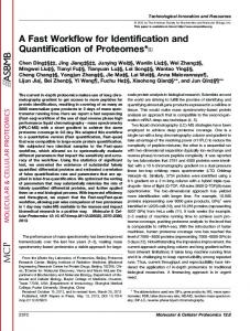
operations. If K 2n0 , the ratio of our time complexity to the FCA-OLS algorithm’s is 5/(n0 + 2n0 −1 ), which means ours is faster when n0 > 2. Since the time complexity of the FCA-OLS algorithm grows exponentially with n0 compared to our algorithm, it will be much slower than our algorithm for large n0 . Our experiments demonstrate this observation. B. Space Complexity The space complexity includes the memory required to store the input data, output data, and the intermediate variables used in the computing procedures. All three algorithms have the same requirement for input and output data, so we only discuss the memory requirements for intermediate variables of the algorithms. Both ours and Adamatzky’s algorithms require memory to store the variables {ˆ σ 2 (n), n = 0, · · · , n0 }, {Lk , k = 0 1, · · · , K}, and {rj , j = 0, · · · , 2n0 − 1}. Ignoring the insignificant parts, the space complexity for both algorithms is K + 2n0 . The largest space requirement for the FCA-OLS algorithm is for storing the regressors {Φji (t)}, which takes K · 2n0 memory stores. Comparing the FCA-OLS algorithm with ours and Adamatzky’s, it can be seen that the former has a higher space complexity, exponentially increasing with n0 , in comparison with the latter. VI. E XPERIMENTAL R ESULTS AND D ISCUSSIONS This section presents some experimental results from our algorithm and gives a timing comparison between our algorithm, Adamatzky’s [15] and Billings and Mei’s FCA-OLS [22] algorithms. A. Experiments on Our New Algorithm Three examples are introduced in this section to show the effectiveness of our algorithm. The first considers a simple one-dimensional three-cell neighbourhood cellular automata, which is used to illustrate the algorithm procedure. We consider a right-shift version of Rule 126 CA. The original Rule 126 CA (named by Wolfram [4]) takes Ni = {ci−1 , ci , ci+1 } as the neighbourhood of the ith cell ci , and the state of the ith cell evolves from time t to t + 1 according to the rules in Table I, where xi (t) represents the state of ci at time step t. The right-shift version has the same rules as in Table I but with its neighbourhood shifted ns cells to the right: Ni = {ci+ns −1 , ci+ns , ci+ns +1 }; in this example, we chose ns = 1. Consider the DCA case. Figure 1(a) shows an example of the evolution of the cell states with black representing 1 and


7

TABLE III PARAMETER E STIMATES AND S TATE T RANSFER RULES OF E XAMPLE 1 (DCA), FROM LEFT TO RIGHT j = 0, · · · , 7 θj xi (t) xi+1 (t) xi+2 (t) xi (t + 1)

0 0 0 0 0

1 0 0 1 1

1 0 1 0 1

1 0 1 1 1

1 1 0 0 1

1 1 0 1 1

1 1 1 0 1

0 1 1 1 0

TABLE IV BIC VALUES FOR D IFFERENT N EIGHBOURHOODS FOR E XAMPLE 1 (PCA)

(a)

(b)

Fig. 1. Evolution of the one-cell right-shift version of the Rule 126 CA in (a) the deterministic case and (b) the probabilistic case; random initialization. TABLE II PARAMETER E STIMATES OF E XAMPLE 1 (DCA)

BY

A LGORITHM 1

j j θ(5)

0 0

1 1

2 0

3 1

4 1

5 1

6 1

7 1

j j θ(5)

8 0

9 1

10 0

11 1

12 1

13 1

14 1

15 1

j j θ(5)

16 1

17 1

18 1

19 1

20 1

21 0

22 1

23 0

j j θ(5)

24 1

25 1

26 1

27 1

28 1

29 0

30 1

31 0

white 0. The first row shows a randomly generated initial state, and each subsequent row is one time step later than the row above. Periodic boundary conditions are used for evolution, i.e. the right-hand neighbour of the last cell is the first cell, the left-hand neighbour of the first cell is the last one, and so on, cyclically. We suppose that no exact neighbourhood is known, and only an a priori maximum neighbourhood size nmax = 7 is assumed to guarantee that all the correct neighbours are included in the neighbourhood. The identification procedure starts by collecting data {yk , xnk }(n = 1, · · · , nmax ) by scanning the image in Figure 1(a) row by row from left to right and top to down, where k is numbered according the order of scanning, so yk = xi (t + 1) is the value of row t + 1 and column i, and {xnk , n = 1, · · · , nmax } are values of nmax columns (centred at column i and ordered in accordance with the neighbourhood described above) in row t. The size of the image is 200 × 200. As each data set comes from two adjacent rows t and t + 1, a total of 199 × 200 = 39, 800 data items are available. After assembling the data, Algorithm 1 is performed to estimate the parameters. The tolerance σT2 is set to be 0 since we are dealing with a DCA. The algorithm ends with a neighbourhood {ci , ci−1 , ci+1 , ci−2 , ci+2 } of size 5 j (although nmax = 7), and the parameter estimates {θˆ(5) ,j = 0, · · · , 31} are shown in Table II. Clearly, the correct neighbours {ci , ci+1 , ci+2 } are included in the output neighbourhood of Algorithm 1, but also included in the output are redundant neighbours ci−1 and ci−2 . The neighbourhood selection procedure described in Section IV-B is then used to eliminate redundant neighbours. Now, the correct neighbourhood {ci , ci+1 , ci+2 } is obtained, and the parameter estimates are shown in Table III. Also shown in Table III are the state

size n 6 5 4 3 2 1

neighbourhood {ci , ci−1 , ci+1 , ci−2 , ci+2 , ci−3 } {ci , ci+1 , ci−2 , ci+2 , ci−3 } {ci , ci+1 , ci+2 , ci−3 } {ci , ci+1 , ci+2 } {ci , ci+1 } {ci+1 }

BIC(n) −3.1264 × 104 −3.1575 × 104 −3.1746 × 104 −3.1831 × 104 −3.0050 × 104 −2.9436 × 104

transition rules, which are obtained according to Eqn. (4). Note the the values in the last row of Table III are exactly equal to those in the first row. Continuing with this example, we consider the PCA case. The same right-shift version of Rule 126 CA is used but the cell state is flipped with a probability p. For example, if {xi (t) = 1, xi+1 (t) = 0, xi+2 (t) = 0}, then xi (t + 1) is 1 in the DCA case, but it is 0 with probability p and 1 with probability 1 − p in the PCA case. Figure 1(b) shows an example of the evolution of the cell states when the flipping probability p is 45%. The triangle patterns seen in the deterministic case are absent. The first steps of the identification procedure for the PCA are the same as that for the DCA, i.e., it starts by collecting data, and applies Algorithm 1 to get initial parameter estimates, and then eliminates redundant neighbours. After these steps, the correct neighbourhood is not necessarily obtained since noise exists in the data, and the BIC neighbourhood selection method described in Section IV-B is used to find the correct neighbourhood. In identifying the CA rules from the data shown in Figure 1(b), the maximum neighbourhood size nmax is still set to be 7, but the tolerance σT2 is set to 0.45, which exactly equals p. After eliminating redundant neighbours, the neighbourhood size is 6, and BIC neighbourhood selection is performed. Table IV shows the BIC values for different neighbourhoods. From the table it can be seen that BIC(3) has the minimum value, so the neighbour size is determined to be 3, and the corresponding neighbourhood is {ci , ci+1 , ci+2 }, which is the same as that obtained in the DCA case. The parameter estimates are also the same as in the DCA case: we have recovered the correct neighbourhood and state transition rules even though the noise level is very high, 45%. Note that here we have assumed that the noise level is known and the tolerance is set to be equal to the noise level. In practice the noise level may be unknown, and the tolerance can not be set in the above way. If the tolerance is set too large, the number of neighbours included from Algorithm 1 may be too small, and some correct neighbours may be not included. On the other hand, if the tolerance is


TABLE VI PARAMETER E STIMATES AND S TATE T RANSFER RULES FOR T HE C ODE 467 CA. k = 0, · · · , 31, FROM TOP LEFT TO BOTTOM RIGHT.

TABLE V S TATE T RANSITION RULES FOR THE C ODE 467 CA

P

xi,j (t) xm,n (t)

Ni,j

xi,j (t + 1)

(a)

8

1 4

0 4

1 3

0 3

1 2

0 2

1 1

0 1

1 0

0 0

0

1

1

1

0

1

0

0

1

1

(b)

Fig. 2. Pattern of the Code 467 CA at time step 22 in (a) the probabilistic case and (b) the deterministic case, starting from a central black pixel.

set smaller, a larger number of neighbours will be included from Algorithm 1, and somewhat more computation is needed during the neighbourhood reduction and BIC neighbourhood selection steps. However, this increased computation is necessary to ensure that the correct neighbours are included and retained. In this example, when σT2 is increased to 0.5, only one neighbour is included from Algorithm 1, and no correct neighbourhood can be obtained. If σT2 is reduced to 0.4, then nmax = 7 neighbours are included from Algorithm 1, and after neighbourhood reduction and BIC neighbourhood selection steps, we still get the correct results. We have performed many experiments with different initial states, and in all cases the correct neighbourhood is chosen after performing BIC neighbourhood selection, if σT2 is set smaller than the noise level. This suggests that in practice, σT2 should be set as small as possible to ensure that the correct neighbourhood is selected. The second example concerns a two-dimensional five-cell neighbourhood totalistic cellular automaton, where the state value xi,j (t+1) of a P cell ci,j at time step t+1 depends only on the total state values (m,n)∈Ni,j xm,n (t) of its von Neumann neighbourhood Ni,j = {(i−1, j), (i+1, j), (i, j−1), (i, j+1)} at the previous time step t, and its own previous state value xi,j (t). Here, we consider a probabilistic version of the Code 467 CA [4]. The original state transition rules of the Code 467 CA are shown in Table V. In this PCA example, the cell state flips with a probability p = 40%. Figure 2(a) shows the pattern (size 91 × 91) of the Code 467 PCA after 22 steps of evolution starting from a single black point in the middle (x46,46 = 1, and other states are 0). The identification procedure follows the same steps as in the first example for identifying the one-dimensional PCA. Let the selected maximum neighbourhood to be a Moore o neighbourhood around the centre cell: Ni,j = {(m, n) : |m − i| ≤ 1, |n−j| ≤ 1}, with size nmax = 9. The data are collected from successive time steps, and at time step t, only the data related to cells {ci,j : |i − 46| < t, |j − 46| < t} are collected.

θk xi,j (t) xi−1,j (t) xi+1,j (t) xi,j−1 (t) xi,j+1 (t) xi,j (t + 1)

1 0 0 0 0 0 1

1 1 0 0 0 0 1

0 0 1 0 0 0 0

0 1 1 0 0 0 0

0 0 0 1 0 0 0

0 1 0 1 0 0 0

1 0 1 1 0 0 1

0 1 1 1 0 0 0


1 0 0 0 1 0 0

1 1 0 0 1 0 0

0 0 1 0 1 0 1

0 1 1 0 1 0 0

0 0 0 1 1 0 1

0 1 0 1 1 0 0

1 0 1 1 1 0 1

0 1 1 1 1 0 1


1 0 0 0 0 1 0

1 1 0 0 0 1 0

0 0 1 0 0 1 1

0 1 1 0 0 1 0

0 0 0 1 0 1 1

0 1 0 1 0 1 0

1 0 1 1 0 1 1

0 1 1 1 0 1 1


1 0 0 0 1 1 1

1 1 0 0 1 1 0

0 0 1 0 1 1 1

0 1 1 0 1 1 1

0 0 0 1 1 1 1

0 1 0 1 1 1 1

1 0 1 1 1 1 1

0 1 1 1 1 1 0

Altogether 16, 214 data items are used for identification. If we set σT2 = 0.4, the five-cell neighbourhood is correctly determined. Table VI shows the parameter estimates and corresponding state transition rules when the neighbours are arranged in the order {ci,j , ci−1,j , ci+1,j , ci,j−1 , ci,j+1 }. Comparing Table VI and Table V, it can be seen that both describe exactly the same state transfer rules—except that the totalistic rules in Table V are simpler in representation. Figure 2(b) shows the pattern at the 22nd step generated by the identified rules with no probabilistic state flipping, starting from a single black point in the middle. This pattern is exactly the same as generated by the Code 467 CA, which validates the identified rules. The third example comes from [4] and shows that our method can also deal with high dimensional CAs and large data sets. It has a 3-dimensional 7-cell neighbourhood: a cell ci,j,k should become black (state value 1) only when exactly one of its 6 neighbours {cm,n,l : |m−i|+|n−j|+|l −k| = 1} were black on the previous step, otherwise it remains unchanged. Note that although the rule statement only mentions 6 neighbours, the central cell ci,j,k is naturally included in the rules, because in the cases it keeps unchanged, the evolved state will depend on its previous state, which makes the neighbourhood size 7. In the experiment, PCA is considered with flipping probability p = 45%, and data are generated according to the above rule, starting from a single black point in the center (x61,61,61 = 1, and other states are 0), and running 30 steps. The identification procedures again follow the steps described above. We assume that a maximal neighbourhood of o Ni,j,k = {(m, n, l) : |m − i| ≤ 1, |n − j| ≤ 1, |l − k| ≤


1, and |m − i| + |n − j| + |l − k| ≤ 2}, which includes nmax = 19 neighbours. The data are collected from successive time steps, and at time step t, only the data related to cells {ci,j,k : |i − 61| ≤ t, |j − 61| ≤ t, |k − 61| ≤ t} are collected. Altogether K = 1, 846, 080 data items are collected, which, considering that nmax = 19, causes the input data {yk , xnk } to comprise 36, 921, 600 numbers. We had set σT2 = 0.45 and even smaller to σT2 = 0.045, but did not obtain the correct neighbourhood. The reason is that the a priori neighbourhood is too large: 219 = 524, 288 parameters or rules need to be identified if all the neighbours are considered, and thus the data is still inadequate to resolve different neighbours. The neighbours selected by Algorithm 1 cannot cover all of the correct neighbourhood. However, when we set σT2 = 0.0045, all 19 neighbours are selected by Algorithm 1, and the following BIC neighbourhood selection procedure correctly determines the 7-cell neighbourhood and corresponding parameters. Since the number of parameters is so large, we do not list the results here. This example again shows that σT2 must be set small to ensure that correct neighbourhood is included from the result of Algorithm 1, especially in the case of large neighbourhoods. It is practical to simply set σT2 = 0, and let nmax to manage stopping Algorithm 1 when one do not know how to set σT2 . The computational cost is also very low. In this experiment on this example, it took less than 2 seconds to generate the correct result when σT2 is set to be 0. Further discussions of time taken by our algorithm come next. B. Computation Time FCA-OLS, Adamatzky’s and our algorithm were implemented in Matlab R2009b to compare their actual computation times. No coding optimization was done for any of these algorithms. We used a Windows 7 platform on a PC with an Intel Xeon Quad-Core 2.4GHz E5530 Processor and 6GB of RAM. The Rule 126 CA was again used here as an example, and only DCA is considered because Adamatzky’s algorithm can only deal with DCA in the formulation discussed in Section II. (We did not use the more complicated 2D Code 467 CA because the FCA-OLS algorithm cannot tackle large neighbourhoods and thus we cannot get enough data for comparison). We have performed many experiments, and have observed similar behaviour in each case. Here we simply use the results of 10 runs with randomly generated initial cell states, which are sufficient to illustrate the algorithm performance. The experimental results shown for Adamatzky’s and our algorithms are based on the average of these 10 runs, while for FCA-OLS algorithm they are divided into two parts: the best-case averages and other case averages. The best case occurs when the forward subset selection method of the FCAOLS algorithm finds the correct neighbourhood and then stops without any redundant neighbours, and the other cases are when a larger neighbourhood other than the correct one is selected before the forward subset selection ends. Three different scenarios are discussed in the following. The first scenario involves the original Rule 126 CA with different initial neighbourhood sizes n0 . The centre of the neighbourhood of a cell ci,j is set to be ci,j itself.

9

Figure 3(a) and (b) show the runtime of FCA-OLS, Adamatzky’s and our algorithms for different n0 with K = 10, 000 data items. Bear in mind that for the FCA-OLS algorithm the result shown is the best-case average, and the runtime can reach 11,272 seconds in the worse-case when n0 = 13. Here we only run the FCA-OLS algorithm for n0 ≤ 13 because when n0 > 13 the algorithm runs out of memory on our computer. It can be seen that the computation times of both Adamatzky’s and our algorithms vary little with changes in n0 , while the time for the FCA-OLS algorithm grows quickly with n0 . In fact, the timing of the FCA-OLS algorithm agrees quite well with the theoretical time complexity we have deduced in Section V-A, which shows it grows exponentially with n0 . The worst-case time complexity of our and Adamatzky’s algorithms grows linearly or quadratically with n0 when K 2n0 (and exponentially otherwise). However in practice, eg., in this scenario, both our and Adamatzky’s algorithms start from the central cell and stop when the neighbourhood size is increased to 3 no matter how large n0 is, so the total time should be almost the same for all n0 ; our experiments agree with this conclusion. The experimental results show that our algorithm is a little bit faster than Adamatzky’s, as predicted by our theoretical analysis. Figure 3(c) and (d) show the runtime ratios of FCA-OLS, and Adamatzky’s algorithm, against ours. Our algorithm is 16–32% faster than Adamatzky’s algorithm, and is more than 34, 000 times faster than FCA-OLS algorithm in its best-case when n0 = 13. If we consider the worst case, we have observed a runtime ratio between FCA-OLS and our algorithm of a factor of more than 12 million in our experiments. The second test also considers the original Rule 126 CA, using a fixed initial neighbourhood size n0 = 11, but with a number of input data items varying from 1, 000 to 10, 000. Figure 4(a) and (b) show the runtime of the algorithms, and Figure 4(c) and (d) shows the runtime ratio of FCA-OL,S and Adamatzky’s algorithm, vs ours. It can be seen that all the three algorithms have a runtime linearly growing with the number of data items, which is consistent with our analyses. Our algorithm here is 12–43% faster than Adamatzky’s algorithm, and is around 2, 200–5, 900 times faster than the FCAOLS algorithm. The third test involves the right-shift Rule 126 CA with shift distances changing from ns = 0 to 9 and K = 10, 000 data items. The initial neighbourhood of a cell is set to be centred at the cell itself with size n0 to guarantee the correct neighbourhood is included, i.e., n0 = 2ns + 3, and the rightmost cell is one of the correct neighbours. Figure 5(a) and (b) show the runtime of the algorithms. It can be seen that the FCA-OLS algorithm behaves as in the first test, since here the increase of ns implies an increase in n0 . The runtime of both our and Adamatzky’s algorithms grows slowly when ns , and hence n0 , is small, and fast when ns is large. This also agrees with our analyses, which shows that the time complexity of both algorithms grows linearly or quadratically with n0 when it is small, and exponentially when it is large. Because both algorithms select neighbours from the centre outwards, in order to include the rightmost cell, all neighbours in the


−3

35

1.5

FCA−OLS

x 10

Adamatzky’s our

1.4

25

time (seconds)

time (seconds)

30 20 15 10

1.3 1.2 1.1 1

5 0 3

5

7

9 11 13 15 initial neighbourhood size

17

19

0.9 3

21

5

7


17

19

21

9 11 13 15 17 initial neighbourhood size

19

21

(a)

(b)

4

3.5

1.35

x 10

3

Adamatzky’s/our FCA−OLS/our

1.3

2.5

time ratio

time ratio

10

2 1.5 1

1.25 1.2

0.5 0 3

5

7


17

19

1.15 3

21

5

7

(c)

(d)

Fig. 3. Computation time for different initial neighbourhood sizes n0 : (a) FCA-OLS algorithm, (b) Adamatzky’s and our algorithm, (c) FCA-OLS / our algorithm, (d) Adamatzky’s / our algorithm. −3

2.5

1.4 1.2

2

time (seconds)

time (seconds)

FCA−OLS

1.5 1

x 10

Adamatzky’s our

1 0.8 0.6 0.4 0.2

0.5 1000 2000 3000 4000 5000 6000 7000 8000 9000 10000 number of data sets

0 1000 2000 3000 4000 5000 6000 7000 8000 9000 10000 number of data sets

(a)

(b)

6000

1.5 FCA−OLS/our

Adamatzky’s/our

1.4 time ratio

time ratio

5000 4000

1.3

3000

1.2

2000 1000 2000 3000 4000 5000 6000 7000 8000 9000 10000 number of data sets

1.1 1000 2000 3000 4000 5000 6000 7000 8000 9000 10000 number of data sets

(c)

(d)

Fig. 4. Computation time and comparison for varying numbers of input data items: (a) FCA-OLS algorithm, (b) Adamatzky’s and our algorithm, (c) FCA-OLS vs our algorithm, (d) Adamatzky’s vs our algorithm.

initial neighbourhood need to be explored, which corresponds to the worst case. Figure 5(c) and (d) shows the runtime ratio of FCA-OLS, and Adamatzky’s algorithm, versus ours. Again our algorithm is about 12–58% faster than Adamatzky’s algorithm, and is more than 8, 347 times faster than the FCAOLS algorithm when ns = 5, corresponding to n0 = 13.

In summary, our algorithm is somewhat faster than Adamatzky’s algorithm, and is significantly faster than the FCA-OLS algorithm even in the best-cases for the FCA-OLS algorithm. Another drawback of the FCA-OLS algorithm is that it is also space-consuming, such that when n0 > 13, the algorithm runs out of memory on our computer, while our


40

0.1

30

time (seconds)

time (seconds)

FCA−OLS

20 10

0.08

Adamatzky’s our

0.06 0.04 0.02

0 0

1

2 3 4 5 6 7 neighbourhood shift distance (cells)

8

0 0

9

1


(a)

9

8

9

1.6

FCA−OLS/our

Adamatzky’s/our

8000 time ratio

1.5

6000 4000 2000 0 0

8

(b)

10000

time ratio

11

1.4 1.3 1.2

1


8

9

(c)

1.1 0

1


(d)

Fig. 5. Computation time and comparison for different neighbourhood shift distances: (a) FCA-OLS algorithm, (b) Adamatzky’s and our algorithm, (c) FCA-OLS vs our algorithm, (d) Adamatzky’s vs our algorithm.

algorithm still works even when n0 > 21. VII. C ONCLUSIONS Considerable research has been done on analysing and simulating CAs with known or designed evolution rules. However, the inverse problem of finding CA rules from observed CA evolution patterns has been relatively little tackled. Most early efforts on this issue used genetic algorithms as a tool to learn CA rules from experimental data. Unfortunately, genetic algorithms can be very time-consuming in real applications. Adamatzky’s CA identification algorithms [15] can extract rules fast from observed data, but the neighbourhood identified by them usually contains some redundant cells, which makes the CA rules overly complex. Maeda and Sakama’s heuristic procedure [17] can remove redundant cells, but only DCA is dealt with. Another drawback of Maeda and Sakama’s algorithm for redundant cell removal is that each time a cell is removed, all data needed to be reconsidered, and identification needs to be recomputed. Billings and colleagues developed a series of relatively fast CA rule identification and neighbourhood selection algorithms [18] based on orthogonal least-squares method, but their algorithms are not efficient for large neighbourhoods. This paper gives a new fast algorithm, which is a significant improvement on the current CA identification algorithms. The proposed algorithm is consistently faster than Adamatzky’s algorithm, and more importantly, it provides a unified approach to rule identification and neighbourhood selection for both DCA and PCA, while Adamatzky’s algorithm does not perform neighbourhood selection. Our algorithm removes redundant cells from neighbourhoods simply based on the

parameter estimates, without resorting to reconsidering data, unlike Maeda and Sakama’s algorithm. The Bayesian information criterion has been used in the proposed algorithm to determine neighbourhoods, which is shown through experiments to work well. Compared to Billings’ most recent fast identification algorithm (FCA-OLS), the proposed algorithm is significantly faster, even when the FCA-OLS algorithm runs in its best case, as well as being much more space efficient. R EFERENCES [1] A. Ilachinski, Cellular Automata: A Discrete Universe. River Edge, NJ, USA: World Scientific Publishing Co., Inc., 2001. [2] J. von Neumann, “The general and logical theory of automata,” in Cerebral Mechanisms in Behavior - The Hixon Symposium, L. Jeffress, Ed. New York: John Wiley & Sons, 1951, pp. 1–31. [3] S. Wolfram, Cellular Automata and Complexity: Collected Papers. Boulder, Colorado, USA: Westview Press, 1994. [4] S. Wolfram, A new kind of science. Champaign, Ilinois, USA: Wolfram Media Inc., 2002. [5] N. Ganguly, B. K. Sikdar, A. Deutsch, G. Canright, and P. P. Chaudhuri, “A survey on cellular automata,” Centre for High Performance Computing, Dresden University of Technology, Tech. Rep., Dec. 2003. [6] J. Shan, S. Alkheder, and J. Wang, “Genetic algorithms for the calibration of cellular automata urban growth modeling,” Photogrammetric Engineering & Remote Sensing, vol. 74, no. 10, p. 12671277, 2008. [7] E. Sapin, L. Bull, and A. Adamatzky, “Genetic approaches to search for computing patterns in cellular automata,” IEEE Computational Intelligence Magazine, vol. 4, no. 3, pp. 20 –28, 2009. [8] P. L. Rosin, “Image processing using 3-state cellular automata,” Computer Vision and Image Understanding, vol. 114, no. 7, pp. 790 – 802, 2010. [9] N. Packard, “Adaptation toward the edge of chaos,” in Dynamic Patterns in Complex Systems, J. Kelso, A. Mandell, and M. Shlesinger, Eds. Singapore: World Scientific, 1989, pp. 293–301. [10] F. C. Richards, T. P. Meyer, and N. H. Packard, “Extracting cellular automaton rules directly from experimental data,” Phys. D, vol. 45, no. 1-3, pp. 189–202, 1990.


[11] M. Mitchell, J. P. Crutchfield, and R. Das, “Evolving cellular automata with genetic algorithms: A review of recent work,” in Proceedings of the First International Conference on Evolutionary Computation and Its Applications (EvCA96). Russia: Russian Academy of Sciences, 1996. [12] Y. Yang and S. Billings, “Extracting Boolean rules from CA patterns,” IEEE Transactions on Systems, Man, and Cybernetics, Part B: Cybernetics, vol. 30, no. 4, pp. 573–580, Aug. 2000. [13] Z. Pan and J. Reggia, “Artificial evolution of arbitrary self-replicating structures,” Journal of Cellular Automata, vol. 1, no. 2, pp. 105–123, 2006. [14] P. Rosin, “Training cellular automata for image processing,” IEEE Transactions on Image Processing, vol. 15, no. 7, pp. 2076–2087, July 2006. [15] A. Adamatzky, Identification of Cellular Automata. London, UK: Taylor & Francis, 1994. [16] A. Adamatzky, “Automatic programming of cellular automata: identification approach,” Kybernetes: The International Journal of Systems & Cybernetics, vol. 26, no. 2, pp. 126–135, Feb. 1997. [17] K.-I. Maeda and C. Sakama, “Identifying cellular automata rules,” Journal of Cellular Automata, vol. 2, no. 1, pp. 1–20, 2007. [18] Y. Zhao and S. Billings, “The identification of cellular automata,” Journal of Cellular Automata, vol. 2, no. 1, pp. 47–65, 2007. [19] Y. Yang and S. Billings, “Neighborhood detection and rule selection from cellular automata patterns,” IEEE Transactions on Systems, Man and Cybernetics, Part A: Systems and Humans, vol. 30, no. 6, pp. 840– 847, Nov. 2000. [20] S. Billings and Y. Yang, “Identification of probabilistic cellular automata,” IEEE Transactions on Systems Man and Cybernetics, Part B: Cybernetics, vol. 33, no. 2, pp. 225–236, 2003. [21] S. Billings and Y. Yang, “Identification of the neighborhood and CA rules from spatio-temporal CA patterns,” IEEE Transactions on Systems Man and Cybernetics, Part B: Cybernetics, vol. 33, no. 2, pp. 332–339, 2003. [22] S. A. Billings and S. S. Mei, “A new fast cellular automata orthogonal least-squares identification method,” International Journal of Systems Science, vol. 36, no. 8, pp. 491–499, 2005. [23] F. Ding, Y. Shi, and T. Chen, “Auxiliary model-based least-squares identification methods for Hammerstein output-error systems,” Systems & Control Letters, vol. 56, no. 5, pp. 373 – 380, 2007. [24] F. Ding, L. Qiu, and T. Chen, “Reconstruction of continuous-time systems from their non-uniformly sampled discrete-time systems,” Automatica, vol. 45, no. 2, pp. 324–332, 2009. [25] F. Ding, P. X. Liu, and G. Liu, “Multiinnovation least-squares identification for system modeling,” IEEE Transactions on Systems, Man, and Cybernetics, Part B: Cybernetics, vol. 40, no. 3, pp. 767 – 778, 2010. [26] F. Ding, P. X. Liu, and G. Liu, “Gradient based and least-squares based iterative identification methods for OE and OEMA systems,” Digital Signal Processing, vol. 20, no. 3, pp. 664 – 677, 2010. [27] F. Ding, G. Liu, and X. Liu, “Partially coupled stochastic gradient identification methods for non-uniformly sampled systems,” Automatic Control, IEEE Transactions on, vol. 55, no. 8, pp. 1976 –1981, 2010. [28] L. He and X. Sun, “Recursive triangulation description of the feasible parameter set for bounded-noise models,” IET Control Theory Applications, vol. 4, no. 6, pp. 985 –992, Jun. 2010. [29] H.-F. Chen, “New approach to recursive identification for ARMAX systems,” IEEE Transactions on Automatic Control, vol. 55, no. 4, pp. 868 –879, Apr. 2010. [30] S. Mei, S. A. Billings, and L. Guo, “A neighborhood selection method for cellular automata models,” International Journal of Bifurcation and Chaos, vol. 15, no. 2, pp. 383–393, 2005. [31] Y. Zhao and S. Billings, “Neighborhood detection using mutual information for identification of cellular automata,” IEEE Transactions on Systems, Man and Cybernetics, Part B: Cybernetics, vol. 36, no. 2, pp. 473–479, 2006. [32] Y. Guo, S. A. Billings, and D. Coca, “Identification of n-state spatiotemporal dynamical systems using a polynomial model,” International Journal of Bifurcation and Chaos, vol. 18, no. 7, pp. 2049–2057, 2008. [33] L. Guo, S. Mei, and S. Billings, “Neighbourhood detection and identification of spatio-temporal dynamical systems using a coarse-to-fine approach,” International Journal of Systems Science, vol. 38, no. 1, pp. 1–15, 2007. [34] M. Esnaashari and M. Meybodi, “A cellular learning automata based clustering algorithm for wireless sensor networks,” Sensor Letters, vol. 6, no. 5, pp. 723–735, 2008. [35] H. Akaike, “A new look at the statistical model identification,” IEEE Transactions on Automatic Control, vol. 19, no. 6, pp. 716–723, 1974.

12

[36] G. Schwarz, “Estimating the dimension of a model,” The Annals of Statistics, vol. 6, no. 2, pp. 461–464, 1978. [37] K. Mao, “Fast orthogonal forward selection algorithm for feature subset selection,” IEEE Transactions on Neural Networks, vol. 13, no. 5, pp. 1218 – 1224, Sep. 2002.

Xianfang Sun received a BSc degree in Electrical Automation from Hubei University of Technology in 1984 and MSc and PhD degrees in Control Theory and its Applications from Tsinghua University in 1991 and the Institute of Automation, Chinese Academy of Sciences in 1994, respectively. He is lecturer at the School of Computer Science & Informatics, Cardiff University. His research interests include computer vision and graphics, pattern recognition and artificial intelligence, system identification and filtering, fault diagnosis and fault-tolerant control. He has completed many research projects and published more than 80 papers. He is on the editorial board of Acta Aeronautica et Astronautica Sinica. He is also a member of the Committee of Technical Process Failure Diagnosis and Safety, Chinese Association of Automation.

Paul L. Rosin is Reader at the School of Computer Science & Informatics, Cardiff University. Previous posts include lecturer at the Department of Information Systems and Computing, Brunel University London, UK, research scientist at the Institute for Remote Sensing Applications, Joint Research Centre, Ispra, Italy, and lecturer at Curtin University of Technology, Perth, Australia. His research interests include the representation, segmentation, and grouping of curves, knowledgebased vision systems, early image representations, low level image processing, machine vision approaches to remote sensing, methods for evaluation of approximation algorithms, etc., medical and biological image analysis, mesh processing, and the analysis of shape in art and architecture.

Ralph R. Martin received the PhD from Cambridge University in 1983, with a dissertation on “Principal Patches”, and since then, has worked his way up from a lecturer to a professor at Cardiff University. He has been working in the field of CADCAM since 1979. He has published more than 170 papers and 10 books covering such topics as solid modelling, surface modelling, intelligent sketch input, vision based geometric inspection, geometric reasoning and reverse engineering. He is a fellow of the Institute of Mathematics and Its Applications, and a member of the British Computer Society. He is on the editorial boards of Computer Aided Design, Computer Aided Geometric Design, the International Journal of Shape Modelling, the International Journal of CADCAM, and ComputerAided Design and Applications. He has also been active in the organisation of many conferences.