{hoeft@cs, schulz@ais, behnke@cs}.uni- bonn.de. Abstract. In semantic scene segmentation, every pixel of an image is assigned a category label. This task can ...
In Proceedings of 37th German Conference on Artificial Intelligence (KI), pp. 80-85, Springer LNCS 8736, Stuttgart, September 2014.
Fast Semantic Segmentation of RGB-D Scenes with GPU-Accelerated Deep Neural Networks Nico Höft, Hannes Schulz, and Sven Behnke
Rheinische Friedrich-Wilhelms-Universität Bonn Institut für Informatik VI, Friedrich-Ebert-Allee 144 {hoeft@cs,schulz@ais,behnke@cs}.uni-bonn.de
In semantic scene segmentation, every pixel of an image is assigned a category label. This task can be made easier by incorporating depth information, which structured light sensors provide. Depth, however, has very di�erent properties from RGB image channels. In this paper, we present a novel method to provide depth information to convolutional neural networks. For this purpose, we apply a simpli�ed version of the histogram of oriented depth (HOD) descriptor to the depth channel. We evaluate the network on the challenging NYU Depth V2 dataset and show that with our method, we can reach competitive performance at a high frame rate. deep learning, neural networks, object-class segmentation Abstract.
Keywords:
1
Introduction
Semantic scene segmentation is a major challenge on the way to functional computer vision systems. The task is to label every pixel in an image with surface category it belongs to. Modern depth cameras can make the task easier, but the depth information needs to be incorporated into existing techniques. In this paper, we demonstrate how depth images can be used in a convolutional neural network for scene labeling by employing a simpli�ed version of the histogram of oriented gradients (HOG) descriptor to the depth channel (HOD). We train and evaluate our model on the challenging NYU Depth dataset and compare its classi�cation performance and execution time to state of the art methods.
2
Network Architecture
We train a four-stage convolutional neural network, which is illustrated in Fig. 1, for object-class segmentation. The network structure, proposed by Schulz and Behnke [1], is derived from traditional convolutional neural networks, but has inputs at multiple scales. In contrast to classi�cation networks, there are no fully connected layers at the top�the output maps are also convolutional. The �rst three stages output maps
Is , C s , Os ,
s = {0, 1, 2}
have input, hidden convolutional, and
respectively. Pooling layers
Ps , Ps0
between the stages
2
Nico Höft, Hannes Schulz, and Sven Behnke I2
I1
I0
C2
O2
P1
P10
C1
O1
P0
P00
C0
O0
O20
Network structure used in this paper. On stage s, I is input, C a convolution, the output, and P a pooling layer. Outputs of stage s are re�ned in stage s + 1, �nal outputs are re�ned from O to O . Solid and dashed arrows denote convolution and max-pooling operations, respectively. Every stage corresponds to a scale at which inputs are provided and outputs are evaluated. Fig. 1.
Os
s
s
i
2
0 2
reduce the resolution of the map representations. The output layer
O20
is the last
stage. The network di�ers from common deep neural networks, as it is trained in stage-wise supervised manner and the outputs of the previous stage are supplied to the next stage to be re�ned. Thus, the lower stages provide a prior for the higher stages, while the simultaneous subsampling allows for the incorporation of a large receptive �eld into the �nal decision. Every layer consists of multiple maps. Input layers have three maps for ZCAwhitened RGB channels, as well as �ve maps for histograms of oriented gradients and depth each (detailed in Section 4). Intermediate layers contain
32
maps.
Convolutions extract local features from their source maps. Following Schulz and Behnke [1], all convolution �lters have a size of The last �lter has a size of
11×11
7×7,
except for the last �lter.
and only re-weights previous classi�cation
results, taking into account a larger receptive �eld. Also note that there are no fully connected layers�the convolutional output layers have one map for every class, and a pixel-wise multinomial logistic regression loss is applied. In contrast to Schulz and Behnke [1], we use rectifying non-linearities
σ(x) = max(x, 0)
after convolutions. This non-linearity improves convergence [2] and results in more de�ned boundaries in the output maps than sigmoid non-linearities. When multiple convolutions converge to a map, their results are added before applying a non-linearity.
3
Related Work
Our work builds on the architecture proposed in Schulz and Behnke [1], which (in the same year as Farabet et al. [3]) introduced neural networks for RGB scene segmentation. We improve on their model by employing rectifying nonlinearities, recent learning algorithms, online pre-processing, and providing depth information to the model.
Fast Semantic Segmentation of RGB-D Scenes with Deep Neural Networks
3
Scene labeling using RGB-D data was introduced with the NYU Depth V1 dataset by Silberman and Fergus [4]. They present a CRF-based approach and provide handcrafted unary and pairwise potentials encoding spatial location and relative depth, respectively. These features improve signi�cantly over the depthfree approach. In contrast to their work, we use learned �lters to combine predictions. Furthermore, our pipeline is less complex and achieves a high framerate. Later work [5] extends the dataset to version two, which we use here. Here, the authors also incorporate additional domain knowledge into their approach, which further adds to the complexity. Couprie et al. [6] present a neural network for scene labeling which is very close to ours. Their network processes the input at three di�erent resolutions using the same network structure for each scale. The results are then upsampled to the original size and merged within superpixels. Our model is only applied once to the whole image, but uses inputs from multiple scales, which involves less convolutions and is therefore faster. Outputs are also produced at all scales, but instead of a heuristic combination method, our network learns how to use them to improve the �nal segmentation results. Finally, the authors use raw depth as input to the network, which cannot be exploited easily by a convolutional neural network, e.g., absolute depth is less indicative of object boundaries than are relative depth changes. A common method for pixel-wise labeling are random forests [7, 8], which currently provide the best results for RGB-D data [9, 10]. These methods scale feature size to match the depth for every image position. Our convolutional network does not normalize the feature computation by depth, which makes it easy to reuse lower-level features for multiple higher-level computations.
4
Pre-Processing 1 only support square input images, we �rst ex-
Since our convolution routines
tend the images with mirrored margins. To increase generalization, we generate variations of the training set. This is performed online on the CPU while the GPU evaluates the loss and the gradient, at no cost of speed. We randomly �ip the image horizontally, scale it by up to
±10%,
shift it by up to seven pixels in
horizontal and vertical direction and rotate by up to
±5◦ .
The depth channel is
processed in the same way. We then generate three types of input maps. From random patches in the training set, we determine a whitening �lter that decorrelates RGB channels as well as neighboring pixels. Subtracting the mean and applying the �lter to an image yields three zero phase (ZCA) whitened image channels. On the RGB-image as well as on the depth channel, we compute a computationally inexpensive version of histograms of oriented gradients (HOG [11]) and histogram of oriented depth (HOD [12]) as follows. For every pixel
p,
we determine its gradient direction
The absolute value of
|αp |
�ve bins at every image location, and weighted by
1
αp
and magnitude
np .
is then quantized by linear interpolation into two of
np .
To produce histograms of
We employ convolutions from the cuda-convnet framework of Alex Krizhevsky.
4
Nico Höft, Hannes Schulz, and Sven Behnke
Network maps, inputs and outputs. First row, ignore mask and ZCA-whitened RGB channels. Second and third row, HOG and HOD maps, respectively. Fourth row, original image, ground truth and network prediction multiplied by ignore mask for reference. Mirrored margins are removed for presentation to save space. Note that HOG and HOD encode very di�erent image properties with similar statistics. Fig. 2.
the orientation strengths present at all locations, we apply a Gaussian blur �lter to all quantization images separately. Finally, the histograms are normalized with the
L2 -hys
norm.
The main di�erence to the standard HOG descriptor is that no image
cells
are combined into a single descriptor. This leaves it to the network to incorporate long-range dependencies and saves space, since our descriptor contains only �ve values per pixel. All maps are normalized to have zero mean and unit variance over the training set. The process is repeated for every scale, where the size is reduced by a factor of two. For the �rst scale, we use a size of
196×196. The teacher maps are
generated from ground truth by downsampling, rotating, scaling, and shifting to match the network output. We use an additional ignore map, which sets the loss to zero for pixels which were not annotated or where we added a margin to the image by mirroring. Sample maps and segmentations are shown in Fig. 2.
5
Experiments
We split the training data set into stage
s,
796
training and
73
validation images. In a
we use the RMSProp learning algorithm with an initial learnrate
to train the weights of all stages below or equal to
s.
10−4 ,
The active stage is auto-
matically switched once the validation error increases or fails to improve. The pixel mean of the classi�cation error over training is shown in Fig. 3. During the �rst two stages, training and validation error behave similarly, while in the �nal
Fast Semantic Segmentation of RGB-D Scenes with Deep Neural Networks
5
classification error
0.6 training set validation set
0.5 0.4 0.3 0.2 0.1
0
500
1000
1500
2000
2500
3000
3500
epoch
Classi�cation error on NYU Depth V2 during training, measured as the mean over output pixels. The peaks and subsequent drops occur when one stage is �nished and learning proceeds to the next�randomly initialized�stage. Classi�cation Results on NYU Depth V2 Method Floor Structure Furniture Props Pixel Acc. Class Acc. Ours without depth 69.1 57.8 55.7 41.7 56.2 56.1 Ours with depth 77.9 65.4 55.9 49.9 61.1 62.0 [6] without depth 68.1 87.8 51.1 29.9 59.2 63.0 [6] with depth 87.3 86.1 45.3 35.5 63.5 64.5 Fig. 3.
Table 1.
stages the network capacity is large enough to over�t.
Classi�cation Performance.
To evaluate performance on the
580
image test
set, we crop the introduced margins, determine the pixel-wise maximum over output maps and scale the prediction to match the size of the original image. There are two common error metrics in the literature, the average pixel accuracy and the average accuracy over classes, both of which are shown in Table 1. Our network bene�ts greatly from the introduction of depth maps, as apparent in the class accuracy increase from
56.1
to
62.0.
We compare our results with
the architecture of Couprie et al. [6], which is similar but computationally more expensive. While we do not reach their overall accuracy, we outperform their
furniture and, interestingly, the rather small props �despite our coarser output resolution. Prediction Speed. We can also attempt to compare the time it takes to promodel in two of the four classes,
cess an image by the network. Couprie et al. [6] report
0.7 s
per image on a
laptop. We process multiple images in parallel on a GPU. With asynchronous pre-processing, our performance saturates at a batch size of able to process
52
64,
where we are
frames per second on a 12 core Intel Xeon at 2.6 GHz and a
NVIDIA GeForce GTX TITAN GPU. Note that this faster than the frame rate of the sensor collecting the dataset (30 Hz). While the implementation of Couprie et al. [6] could certainly also pro�t from a GPU implementation, it requires more convolutions as well as expensive superpixel averaging and upscaling operations. Our network is also faster than random forests on the same task (30.3 fps [10], hardware similar to ours).
6
REFERENCES
6
Conclusion
We presented a convolutional neural network architecture for RGB-D semantic scene segmentation, where the depth channel is provided as feature maps representing components of a simpli�ed histogram of oriented depth (HOD) operator. We evaluated the network on the challenging NYU Depth V2 dataset and found that introducing depth signi�cantly improved the performance of our model, resulting in competitive classi�cation performance. In contrast to other published results of neural network and random-forest based methods, our GPU implementation is able to process images at a high framerate of 52 fps.
References [1]
H Schulz and S Behnke. � Learning object-class segmentation with convolutional neural networks�. In:
[2]
Eur. Symp. on Art. Neural Networks. 2012.
A Krizhevsky, I Sutskever, and G Hinton. � Imagenet classi�cation with deep convolutional neural networks�. In:
cessing Systems. 2012. [3]
Adv. in Neural Information Pro-
C Farabet, C Couprie, L Najman, and Y LeCun. � Scene parsing with multiscale feature learning, purity trees, and optimal covers�. In:
preprint arXiv:1202.2160 [4]
N Silberman and R Fergus. � Indoor scene segmentation using a structured light sensor�. In:
[5]
Int. Conf. on Computer Vision (ICCV) Workshops. 2011.
N Silberman, D Hoiem, P Kohli, and R Fergus. � Indoor Segmentation and Support Inference from RGBD Images�. In:
Vision (ECCV). 2012.
[6]
[8]
Europ. Conf. on Computer
C Couprie, C Farabet, L Najman, and Y LeCun. � Indoor Semantic Segmentation using depth information�. In:
[7]
arXiv
(2012).
CoRR
abs/1301.3572 (2013).
T Sharp. � Implementing decision trees and forests on a GPU�. In:
Conf. on Computer Vision (ECCV). 2008.
Europ.
J Shotton, T Sharp, A Kipman, A Fitzgibbon, M Finocchio, A Blake, M Cook, and R Moore. � Real-time human pose recognition in parts from single depth images�. In:
[9]
Communications of the ACM
(2013).
J Stückler, B Waldvogel, H Schulz, and S Behnke. � Dense real-time mapping of object-class semantics from RGB-D video�. In:
Time Image Processing [10]
Journal of Real-
(2013).
AC Müller and S Behnke. � Learning Depth-Sensitive Conditional Random Fields for Semantic Segmentation of RGB-D Images�. In:
Robotics and Automation (ICRA). 2014. [11]
Int. Conf. on
N Dalal and B Triggs. � Histograms of oriented gradients for human detec-
Computer Vision and Pattern Recognition (CVPR). 2005. Int. Conf. on Intelligent Robots and Systems (IROS). IEEE. 2011. tion�. In:
[12]
L Spinello and KO Arras. � People detection in RGB-D data�. In: