Mar 13, 1996 - tables of upper and lower bounds of the exponential and logarithm func- ...... After step 3c, there is a real numbers r; u 2 0;1) such that n + r =.
Fast, Sound and Precise Narrowing of the Exponential Function
Timothy Hickey�and Qun Ju Michtom School of Computer Science Volen Center for Complex Systems Brandeis University, Waltham MA, 02254 March 13, 1996 Abstract
In this paper we present an algorithm for narrowing the constraint = ex . The algorithm has been designed to be fast by using only IEEE multiplication. The main di�culty is to design algorithms which soundly, rapidly, and precisely compute upper and lower bounds on ex and ln(y). We prove that our algorithms are correct and produce upper and lower bounds which di�er by at most 2 ULP. The method we describe is a modi cation of the standard range reduction algorithm found in the literature, but is considerably more complex due to the necessity of guaranteeing that the algorithm computes tight upper and lower bounds for all inputs x. The algorithm assumes that the arithmetic operations (+,-,*,/) are implemented in hardware and that rounding control can be speci ed by the user (e.g. the IEEE 754 speci cations of single, double, and extended precision arithmetic all satisfy these assumptions). The bounds for exp and log are computed using the native oating point arithmetic to guarantee soundness and speed. Precision is attained by using precomputed tables of upper and lower bounds of the exponential and logarithm functions at predetermined points. Experiments reveal that in an experiment with N random inputs, the fraction which are 2 ULP apart is approximately N=2M ?2 and our analysis suggests that in general this fraction will be inversely proportional to the size of the table. In the nal remarks we discuss a method for extending this technique to the narrowing of the trigonometric and hyperbolic functions. y
� This research was partially supported by NSF grant CCR-9403427
1
1 Introduction One of the most exciting advances in constraint logic programming over the last few years has been the incorporation of the relational interval arithmetic constraint solving algorithm in CLP systems (see CLP(BNR) [15] and CLP(F) [10]). These new CLP languages allow the user to solve complex arithmetic constraints involving not just the algebraic functions (+,-,*,/), but a wide range of other functions as well [2]. One of the distinguishing features of CLP(intervals) interpreters is that they are sound, i.e., if S is any set of constraints on a set V of variables, and if the interpreter narrows the ranges of the variables in V , then all solutions to the system S are guaranteed to be contained in the narrowed intervals. In other words, CLP(intervals) interpreters use algorithms which reduce interval widths and never omit any solutions. To prove the soundness of a CLP constraint solver which is based on interval arithmetic, it is necessary and su�cient to prove that the narrowing algorithms associated to each primitive constraint are sound. For the narrowing of addition and multiplication, this is a relatively straightforward problem, since the IEEE 754 standard [11] for double precision arithmetic allows the user to specify the rounding mode for the primary operations (+,-,*,/) and the square root. In this paper we show how to implement a sound narrowing algorithm for constraint y = xx . In the nal remarks we describe our current e�orts at extending this method to the trigonometric, and the hyperbolic function constraints. From a practical point of view, the narrowing operators should be not only sound but also fast, since they are the dominant operation in an interval arithmetic constraint solving system. They should also be precise, that is, the upper and lower bounds returned by the narrowing procedure for a relation should be as close as possible to the mathematically tightestest upper and lower bounds. Finally, the space taken by the narrowing procedure should be relatively small. There is a natural tradeo� between speed, space usage, and precision of the narrowing procedures. We begin with a quick description of the IEEE 754 standard for oating point arithmetic, which motivates our more general \ oating point" domain. We then prove some Propositions concerning the result of evaluating certain types of expressions with various rounding modes selected. Finally, we describe how to narrow the relation y = ex , rapidly, soundly, and precisely using only oating point arithmetic operations. This narrowing algorithm relies on an algorithm for rapidly calculate precise upper and lower
oating point bounds on ex and ln(x) for oating point numbers x. For the exp (resp. ln) function we prove soundness of the upper and lower bound algorithms, and we also prove that the computed bounds for ex usually di�er by one unit in the last place (ULP) and at worst di�er by two ULPs. These results are supported by experimental evidence. Finally, we provide a brief overview of what is required to extend the method 2
employed for narrow ex to the trigonometric and hyperbolic relations.
2 Related work There are several di�erent approaches to the problem of soundly implementing narrowing for special functions such as exp and ln. We consider three alternate approaches in this section. The easiest method to implement is to use a sound interval arithmetic package [14] to evaluate the Taylor polynomial (with a sound estimate of the remainder term) of the function f(x) being computed. This method will compute both an upper and lower bound simultaneously and the code is simple and easily veri ed to be correct, assuming the correctness of the underlying interval arithmetic package. The main disadvantages of this approach are � each interval operation requires a large number of primitive tests and operations, resulting in a considerable slow down � it may produce highly imprecise results for large x, since it requires a large number of terms of the Taylor polynomial. The second drawback can be attacked by using the standard range reduction methods (described below), but the deleterious e�ect on the execution speed is unavoidable with this approach. The next simplest approach is to use a multiprecision arithmetic package such as PARI [3]. The main disadvantage of this approach is again that an unavoidable slowdown in execution speed will result since each multiprecision arithmetic operation requires several machine cycles to execute. Another approach is to simply use a standard numerical methods approach [7, 8] provided one can prove that the error in the computed result is at most k unites in the last place (ULP). Many math packages use a rational or polynomial approximation to the function when the argument is small and use standard techniques for reducing the range when the argument is large. We will in fact use variants of these standard techniques, where we modify them so that they produce upper (or lower bounds) and remain highly accurate. If one is lucky enough to have a fast numerical routine with a guaranteed maximum bound on the error in terms of a small number k of ULP, then one can compute upper and lower bounds for ex by calling that exp(x) function and then adding or subtracting k ULP to obtain the upper or lower bound. There are two main problems with this approach. The rst problem is that it is often di�cult to nd a proof that the computed value of the function is at most k ULP away from the true value of the function. For scienti c computing it usually su�ces to have an implementation in which the error (in ULP) is small a large percent of the time, and this can easily be checked experimentally. 3
The second problem is that, even in the best case when there is a proof that the error is at most 1/2 ULP, if we let f = exp(x) be the compute value, then we know that the di�erence between the real value g = ex and f is at most 1 ULP, but we don't know if f if above or below g, so to get sound bounds f? < ex < f+ , we must let f? be the oating point number preceeding f and let f+ be the one following f. Thus, even in this best case, we get an error of at least 2 ULP.
3 Preliminaries
3.1 IEEE Arithmetic and Sound Interval Arithmetic
Floating-point arithmetic is ubiquitous in scienti c computing, but as is wellknown, most oating-point operations produce mathematically incorrect results due to the limited number of bits allowed in the representation of real numbers. Luckily, most modern computers rely on the IEEE 754 standard to determine how these unavoidable roundo� errors should be handled. Thus, although all machines produce mathematically incorrect results, if they use the IEEE standard, then they produce the same incorrect results, at least for the basic arithmetic operations (+.-.*,/). The standard does not however address the roundo� error of the special functions (exp,log,sin,cos,sinh, bessel functions, etc.). Our goal in the following section is to show how to compute upper and lower bounds for these functions with a provably small error using the arithmetic operations as described by the IEEE standard. A good introduction to oating point arithmetic is Goldberg's survey [9].
3.2 Overview of the IEEE 754 standard
IEEE 754 is a standard for binary oating-point arithmetic, which speci es the precise layout in di�erent precisions such as single and double precisions. According to IEEE 754 standard, which for simplicity we shall call the IEEE standard through out this paper, Numbers in the binary oating-point formats are composed of 3 elds: 1. (Sign Field) A 1-bit sign s. 2. (Exponent Field) A biased exponent e1 e2 � � � em , where m = 11 for double precision (m = 8 for single precision). We de ne E = e1 e2 � � � em ? bias, where bias = 2m?1 ?1, It is clear that Emin = 0?bias = ?bias = 2m?1 ?1, Emax = 2m ? 1 ? bias = 2m?1 . 3. (Fraction Field) A fraction x1x2 � � � xn. where n = 52 for double precision (n = 23 for single precision). De ne f = 0:x1x2 � � � xn. 4
The value of the number X represented by a single or double precision bit string is determined as follows: 1. (normal case) when Emin < E < Emax : X = (?1)s 2E 1:x1x2 � � � xn 2. (denormalized case) when E = Emin: X = 0 if if x1 x2 � � � xm = 00 � � � 0, else X = (?1)s 2E 0:x1x2 � � � xn 3. (NaN and 1 case) when E = Emax : X = 1 if x1 x2 � � � xm = 00 � � � 0, else X is NaN Observe that two di�erent binary bit strings represent di�erent oating-point number(including +1, ?1) except for the case of NaN and zero. There are many di�erent data formats for the NaN. There are exactly two representations for number 0 because s can be either 0 or 1, we call it +0, ?0 respectively. +0 and ?0 are the same in all arithmetic operation, except one case 1=0. Strictly saying, if the division-zero exception (see next paragraph) is disable (which exactly is the default situation), 1= + 0 will return +1, 1= ? 0 willreturn ?1. The IEEE standard requires that the exceptions for invalid operation, divisionby-zero, over ow, under ow, and inexact should be capable of being enabled/disabled separately or in groups. Also there are 4 rounding modes, i.e, round toward nearest(RN), zero(RZ), +1(RP), and ?1(RM). The rounding operation is speci ed by IEEE standard that rounding takes a number regarded as in nitely precise and, if necessary, modi es it to t in destination's format while signaling the inexact exception. Except for binary-decimal conversion, operation such as add, subtract, multiply,divide, square root, round to integer, shall performed as if it rst produced an intermediate result correct in nite precision and with unbounded range, and then round that result according to the current rounding mode. It is obvious that the operations, such as oating-point compare, absolute value, negative operation, are exact.
3.3 General Floating Point Numbers
In this section we describe the classes of oating point numbers considered here. We use this class so that the results may be extended to hardware that supports larger oating point numbers that the standard double precision (e.g. 96 bit, 128 bit, or more). The algorithms described in this paper are designed to compute upper and lower bounds on the elementary functions while using only the generalized oating point arithmetic described in this section. The set of oating point numbers will be denoted R = R(emax; emin; F) where F is the number of bits used to represent the fractional part of the number and [emin; emax] is the range of base 2 exponents allowed in this representation. If we let E denote the number of bits needed to represent the exponent, then E = 5
ceiling(log2 (emax ? emin)). A oating point number x can then be represented by three bit strings s (the sign bit), e (the exponent bits), and f (the fraction bits) of lengths 1, E, and F and the representation is the obvious generalization of IEEE 754, where we simply change the size of the exponent and fraction elds of IEEE 754 from (11,52) to (E,F). In this new context, we use the same de nitions of denormalized numbers, biased exponents, positive and negative in nity, and NANs. We let R denote the set of real numbers and we let �? (resp. �+ ) denote the \rounding mode map" which maps R to R by rounding down (resp. up) to the nearest element of R: �? : R ! R �? (x) = sup(r 2 R; r � x) �+ : R ! R �? (x) = inf(r 2 R; x � r) We let �; ; ; � denote the oating point implementations of the standard arithmetic operators +; �; ?; =. When the rounding mode has been set to round toward positive in nity, we indicate this by placing a bar over the operator, as with �; � ; �� ; � . Similarly, an underbar is used to denote rounding toward negative in nity. Thus, a�b = �? (a + b) a b = �? (a ? b) a b = �? (a � b) a�b = �? (a=b) a�b = �+ (a + b) a � b = �+ (a ? b) a � b = �+ (a � b) a�� b = �+ (a=b) Recall also that R is the union of a nite set of real numbers with the nonnumbers f+1; ?1; nang. We will let � denote the successor function of R: �(x) = inf(fr 2 R : x < rg) if x 2 R ? f+1; nang and for the non-numbers we de ne �(+1) = +1, �(nan) = nan. We also de ne �(x) to be a unit in the last place (ULP) of a number x 2 R, that is: �(x) = �(jxj) ? jxj This is only de ned for numbers x such that �(jxj) 62 f+1; nang. When we say that a and b are k ULP apart, we will mean precisely that �k (a) = b That is, we can get from a to b by successively applying the operator which adds one unit in the last place: x 7! x + mu(x) Observe that the concept of 1 ULP depends on base 2 exponent of the oating point whose unit in the last place is being considered. If x and y are to oating 6
points with the same base 2 exponent, i.e., �(x) = �(y), then they will have the same ULP. We will de ne �( ) for any real number by �( ) = �(�? (j j)) Thus, if lies between two oating point numbers, x and y, then �( ) will be the minimum of �(x) and �(y).
3.4 Some properties of arithmetic using IEEE rounding modes
Note that setting the rounding mode to round toward minus in nity does not guarantee that every assignment v = E will produce a lower bound for the expression E. For example, if x = ?x0 is negative and y is positive, then the assignment v = x � (1+y) will proceed by evaluating 1+y and rounding toward minus in nity to get 1+y ? e1. It will then multiply this by x and round toward minus in nity again to get: x (1�y) = x � (1 + y ? e1) ? e2 = ?(x0 � (1 + y)) + x0 � e1 ? e2
Thus, depending on the relative sizes of the errors e1; e2 and x, the result stored in v could be either above, below, or equal to the true value of E. There are however two special cases where the result of evaluating an expression E with the rounding set to RM (resp. RP) has the same e�ect as evaluating the expression in \in nite precision" arithmetic and then rounding toward minus in nity (resp. plus in nity). We describe these two useful cases in the following two propositions.
Proposition 1 Let a ; : : :; an 2 R be oating point numbers such that for each i, ai � (ai + : : : + an ) � 0. Then, a �(a � : : :(an? �an ) : : :) = �?(a + : : : + an) a �(a � : : :(an? �an) : : :) = � (a + : : : + an) Proposition 2 Let a ; : : :; an 2 R be oating point numbers such that for each i, jai j � 2jai + : : : + anj. Then, a �(a � : : :(an? �an ) : : :) = �?(a + : : : + an) a �(a � : : :(an? �an) : : :) = � (a + : : : + an) 1
+1
1
1
2
1
2
1
+
1
1
1
+1
1
2
1
1
2
1
1
+
1
These two propositions allow us to conclude that by properly setting the rounding mode to round toward positive (resp. negative in nity) the result of evaluating certain decreasing sums of oating point numbers will be an upper bound (resp. lower bound) of the sum which is precise to the last bit. 7
Corollary 1 Let a1 ; : : :; an 2 R be oating point numbers as in either of the two previous propositions, and let v? = a1�(a2 � : : :(an?1�an ) : : :)v+ = a1 �(a2 � : : :(an?1 �an) : : :) Then, v? < v+ are consecutive oating point numbers, i.e. �(v? ) = v+ . The two propositions above follow easily from the following lemma by induction on n. The n = 2 case is trivially true. Assuming now the propositions are true for n ? 1, we get the induction case from the lemma by setting = a2 + a3 + : : : + a n and a = a1. Lemma 1 Let a 2 R be any oating point number and let 2 R be any real number such that either a � � 0 or if jaj > 2j j, then �? (a + ) = �? (a + �? ( )) �+ (a + ) = �+ (a + �+ ( ))
Proof. Let us rst prove the following claim: Claim 1 that if s 2 f+; ?g then
�s(a + ) = �s (a + �s( ))
is true if
�s(a + ) ? a 2 R In the case where s = +, we have c = �+ (a + ) � �+ (a + �+ ( )) = d If the lemma is false then we must have c < d. Thus, from the de nition of �+ we get a + � c < a + �+ ( ) � d And if we subtract a from both sides we get � c ? a < �+ ( ) � d Observe now that if c ? a 2 R, then by the de nition of �+ we must have �+ ( ) = c ? a 8
which is a contradiction. The case where s = ? can be proved in the same way. We can also reduce to the previous case using the fact that �? (a) = ?�+ (?a) c ? a 2 R , ?(c ? a) 2 R To conclude the proof of the lemma, we will show the following:
Claim 2 Let a 2 R and let 2 R, and let s 2 f+; ?g, then �s(a + ) ? a 2 R is true if
� a � � 0, or � jaj � 2j j Consider rst the case where a � � 0. If a = then a+ = 2a 2 R and the lemma is trivially true, so we may assume that a > . In this case, let = a+ and let c = �s (a+ ) and � = c ? a. Observe that 2a � c � a � c ? a � 0. Thus, if �(c) denotes the base two exponent of c, then �(c) � �(a) � �(c ? a). Thus, if we let �(a) be the power of two which denotes one unit in the last place of a, then �(c) � �(a) � �(c ? a). But c ? a is formed from bit-by-bit subtraction and so �(c ? a) = �(a). Since �(c ? a) � �(a), we see that c ? a can be expressed with a fractional part of at most F bits and since the last non-zero bit in c ? a is in no smaller a position than �(a), this holds even if �(c ? a) < emin and c ? a is denormalized. Consider now the case where jaj � 2j j. We may assume without loss of generality, that a > 0 and < 0. Again letting c = �s (a + ), we nd that a � c � a=2 � a ? c � 0 Thus, we see that �(c) 2 �(a)+[0; ?1] and �(a ? c) � �(a) ? 1. Since �(a ? c) � �(c) we must be able to represent a ? c with a fractional part of at most F bits and with the position of its last nonzero bit no smaller than �(c). Thus, a ? c 2 R.
4 Sound Narrowing for exp and log In this section we describe fast, sound and precise implementations of the the procedure: BOOLEAN narrow_exp(INTERVAL *X,INTERVAL *Y);
9
boolean narrow_exp(interval *x, interval *Y){ boolean val=true; intersect(Y,exp_clp(lo,X->lo),exp_clp(hi,X->hi),&val); intersect(X,log_clp(lo,Y->lo),log_clp(hi,Y->hi),&val); return(val); } void intersect(interval *X, double vlo, double vhi, boolean *val) { if (!(*val)) return; if (vhi < X->hi) X->hi = vhi; if (X->lo < vlo) X->lo = vlo; *val = (X->lo hi); }
Figure 1: Procedure narrow exp which accepts two intervals X and Y whose endpoints are oating point numbers (possibly in nite). The narrow exp procedure narrows the intervals X and Y in such a way that if x 2 X and y 2 Y before the call and if ex = y, then x and y will still belong to the narrowed intervals after the call. If the intervals are narrowed to the empty interval then narrow exp returns FALSE otherwise it returns TRUE. Since exp and log are inverse functions we can implement narrow log(X,Y) as a call to narrow exp(Y,X). Moreover, since they are both monotone increasing functions the narrowing procedure is particularly simple and is shown in Figure 1. The procedure void intersect(INTERVAL *X,double lo,double hi,BOOLEAN *v)
intersects the interval *X with the interval [lo; hi] and stores the value back in X provided the result is non-empty and *v = TRUE, otherwise it returns with *v = FALSE. The two functions double exp_clp(int lohi,double x); double log_clp(int lohi,double x);
compute upper and lower bounds on ex and ln(x), that is, for all x we have: exp_clp(lo,x) max real or x e < min real, we can return the appropriate upper and lower bounds without further computation. We may now assume that x 2 [log min real; log max real] � [log2(min real); log2 (max real)] � [?2E ?1; 2E ?1] where we have used the fact that log2 (x) > ln(x) and that the base 2 exponents of min real and max real are within the stated bounds. Step 2. Here we set the rounding mode which applies to all arithmetic operations in the rest of the procedure. When computing an upper bound for 20
ex (i.e., when hilo = HI) we set the mode to round up. When computing lower bounds, we set the mode to round the result of each operation down. One of the important features of our system is that we use a single rounding mode throughout. Let s be 1 (resp. -1) if hilo = HI (resp. LO), then we can express the result of an arithmetic operation under the current rounding mode as follows: a � b = (a + b) � (1 + s � v) a b = (a � b) � (1 + s � v) a b = (a ? b) � (1 + s � v) a � b = (a=b)(1 + s � v) where v 2 [0; 2?F ] provided the result is a nite number which is not denormalized. Step 3. These lines of code are designed to nd the decomposition x+s � � = a + i=2m + n � ln(2) for some very small positive epsilon. We will now prove the following lemma. Lemma 2 At the end of Step 3, the integers n and i and the oating point numbers a and x have the following properties � If jxj < 2?M +1 , then a = x and i = n = 0, � If n = 0 and jxj � 2?M +1, then x = a + i=2m i 2 [0; 2M ] a 2 [0; 2?M )
� If n 6= 0, and jxj � 2?M +1 , then for some � 2 [0; 2?F ?M +1], we have x + s � � = a + i=2M + n � ln(2) n 2 [?2E ; 2E ] i 2 [0; (7=8)2M ] a 2 [0; (5=4)2?M +1) Lets begin by examining step 3a. If this conditional is true, then we simply set i = n = 0 and a = x and the lemma is true in this case. We can now assume that the condition is false and so jxj � 2?M +1 . After step 3b, there is an �1 such that ln2 est = ln(2) + sx �1 �1 2 [2?B?1; 2?B ] where sx is the sign of x (i.e., 1 if x � 0 and -1 otherwise). After step 3c, there is a real numbers r; u 2 [0; 1) such that n + r = ln(2) x+ s � (1 + su2?F ) x1 and n is an integer. At this point, if n = 0 then we must have x 2 (ln(2) + 2?B )=(1 ? 2?F )[0; 1) � [0; 0:75) 21
where we have used the assumption that F � B � E � 12 to make a very rough estimate of the interval containing x. In the case where n = 0, we will let y = x in step 3d and in steps 3e-3h, using the fact that M < F, we nd an integer i and a oating point number a such that the following relation holds with no roundo� error: x = a + i=2M as was claimed in the lemma. We can now assume that n 6= 0 and jxj � 2?M +1 . We will show that the
oating point number y computed in step 3d must satisfy: y 2 [2?B?2 ; 2?M +1] Recall rst from the de nition of precomputed constants that ln2a = ln2 a[hilo2] = ln(2) + sx u2?C ?1 for some u 2 [0; 1) and where sx is, again, the sign of x (which comes in because of the index hilo2). Moreover, because of the fact that ln2a is a C + 1 bit binary number, and n is a binary number of at most E bits, we see that the product n � (?ln2a) can be computed exactly on the processor (using the fact that E + C � F). We can now begin our estimate of y: y = (x + n(?ln2a))(1 + su2?F ) ? � ? F ? C ? 1 = (n + r)(ln(2) + sx �1) ? su2 x ? n(ln(2) + sx u2 ) (1 + su2?F ) ? � = rln2 est + nsx �1 + u2?C ?1 ? jx=njsu2?F � [2?B?1 ? 2?C ?1 ? 2?F +1 ; ln(2) + 2?B + 2E ?B + 2E ?C ?1 + 2E ?F +1 ] � [2?B?2; ln(2) + 1=8] � [2?B?2 ; 7=8] where we have made use of the fact that jx=nj � 2, and the fact that F � C � B + 3 > B � E + 4 > E � 11, ?B � ?15, E ? B � ?4, E ? C ? 1 � ?5, E ? F ? 1 � ?5 and ln(2) < 3=4. In step 3e we nd the integer i such that i ; i + 1] y 2 [ 2M 2M In step 3f, we adjust i so that if y < 2?M (or n = 0 which we considered earlier); otherwise, we decrement i so that y 2 [ 2iM ; i2+M1 ) + 1=2M In step 3e, we subtract the (exactly representable) oating point number i=2M from y to get a1. In the case where y < 2?M , then we must have a1 = y ? i=2M 2 [2?B?2; 2?M ) 22
If y � 2?M , then we may have some error when making this subtraction, but since a1 � 1=2M , this error is bounded by 2?F ?M , so we have: a1 = (y ? i=2M )(1 ? su2?F ?M ) 2 [2?M ; 2?M +1) Finally, in step 3f, we add n*(-ln2 b[hilo2]) to a1 to get a. In the case where y � 1=2M , we know that a1 > 2?M and so a 2 [2?M ? 2E ?C ; 2?M +1 + 2E ?C ] � [2?M ?1; 54 2?M +1 ] where we have used the fact that E + M + 1 < C to infer that 2E ?C < 21 2?M In the case where y < 2?M , we have a 2 [2?B?2; 2?M ] + [?2E ?C ; 2E ?C ] � [0; 2?M +1] This proves the lemma. Step 4 In this step we compute a Taylor series approximation z to ea ? 1. The analysis here is a little subtle because we must show that these few lines of code compute a true upper or lower bound (depending on hilo) for all a 2 [?2?M +1; 2?M +1]. In step 4a, we set aa to be an upper or lower bound on a � a (depending on hilo) We also set d to the smallest odd number with d � expdeg. Thus, aa = a2 (1 + su2?F ) d � expdeg for some u 2 [0; 1). In step 4b, we compute the Horner rule term corresponding to the remainder term for the Taylor polynomial of degree d+1, this should be an estimate of e�a ad+2 =(d + 2) and since we assume � 2 [0; ln(2)], we get: e�a ad+2 =(d + 2) 2 2s ad+2 =(d + 2) where s is the rounding mode (1 for hi, -1 for lo). So, for some u 2 [0; 1) we have e�a ad+2 =(d + 2) = z(1 ? s�) � = (2 ? 1=2)ad+2 =d + 2 In steps 4c,d we compute the value of the Taylor polynomial with remainder using the Horner rule, by iterating the assignment: z = ((z � 1) � (j � 1) aa � a) � j; Although it is not obvious, it is straightforward to check that as long as z 2 [0; 1) if this expression is evaluated with a rounding mode set to round down (RM), then the result will be a lower bound on the true value computed by the Horner rule, and if the rounding mode is set to round up (RP), then the result will be an upper bound. To see this, we consider the evaluation of this assignment 23
using interval arithmetic given intervals for aa and z, and assuming that a and j are exact: [z? ; z+ ] (([z? ; z+ ] � 1) � ([j; j] � 1) [aa? ; aa+ ] � [a; a]) � [j; j] and using the fact that that aa? and z? + 1 will always be positive, we get = [((z? �1)�(j �1) aa? �a)�j; ((z+ �1)�� (j �1) � aa?�a)�� j] which shows that we can compute lower bounds using RM and upper bounds using RP. Next we estimate the error between the computed value of z and the actual value of ea ? 1. Claim 3 Let zs be the oating point value computed in step 4, where as usual, s denotes the rounding mode, and sa denotes the sign of a, then zs = �s((ea ? 1)(1 ? sa s22?M ?F )) and hence if n = 0, then z? < ea < z+ and z+ is at most 2 ULP larger than z? .
Proof. [of claim] Let zd denote the initial value assigned to z, and let zj +2
denote the value assigned to z inside the loop when the index variable has value j. Thus, for j 2 [1; d] we have z2j ?1 = ((z2j +1 + 1)=(2j) � aa + a)=(2j ? 1); Similarly, let wd+2 = e�a ad+2 =(d + 2) denote the actual remainder term in the (Horner form of the) Taylor polynomial for ea , and de ne w2j ?1 by w2j = (w2j +1 + 1)=(2j) � a2 w2j ?1 = (w2j + 1)=(2j ? 1) � a So that ea = 1 + w1 , and we have w2j ?1 = ((w2j +1 + 1)=(2j) � a2 + a)=(2j ? 1) We will compute an estimate for �j de ned by w2j +1 = z2j +1(1 ? s0 �2j +1, where s0 = ssz where s is the rounding mode and sz = sa is the sign of z. Let's estimate z2j ?1 ? w2j ?1. z2j ?1 = (((w2j +1(1 ? s0 �)) � 1) � (2j) aa � a) � (2j ? 1) = (((w2j +1 (1 ? s0 �2j +1)) + 1)(1 ? su2?F ) � (2j) aa � a) � (2j ? 1) = (((w2j +1(1 ? s0 �2j +1)) + 1)=(2j)(1 ? su2?F )2 aa � a) � (2j ? 1) = (((w2j +1(1 ? s0 �2j +1)) + 1)=(2j) � aa(1 ? su2?F )3 � a) � (2j ? 1) = (((w2j +1(1 ? s0 �2j +1)) + 1)=(2j) � a2(1 ? su2?F )4 � a) � (2j ? 1) = (((w2j +1 (1 ? s0 �2j +1)) + 1)=(2j) � a2(1 ? su2?F )4 + a)=(2j ? 1)(1 ? s0 u0 2?F )2 = (((w2j +1) + 1)=(2j) � a2 (1 ? s�02j ) + a)=(2j ? 1)(1 ? s0 u0 2?F )2 24
where (1 ? s�02j ) = (1 ? ssz �2j +1w2j +1=(1 + w2j +1))(1 ? su2?F )4 We can use the Taylor remainder to estimate sz wj +2 and we get 0 � sz w2j +1 � 2sz a2j +1=(2j) � 22(2j +1)(1?M )=(2j) � 2(2j +1)(1?M ) Moreover we assume that F � 52 and jaj < 2?M +1, so we get �02j < �2j +122(2j +1)(1?M )+1 Continuing, we get z2j ?1 = (w2j (1 ? s�02j ) + a)=(2j ? 1)(1 ? s0 u02?F )2 = (w2j ?1 ? s�02j w2j =(2j ? 1))(1 ? su02?F )2 = w2j ?1(1 ? s�02j w2j =((2j ? 1)w2j ?1)))(1 ? su02?F )2 and we can estimate w2j =w2j ?1 by w2j =w2j ?1 = e�1 a2j =(2j)=(e�2 a2j ?1=(2j ? 1)) = e�3 a(1 ? 1=(2j)) where j�ij � jaj � 21?M , so sz w2j =w2j ?1 2 [0; 22?M ] Thus, we get z2j ?1 = w2j ?1(1 ? ssz �02j 21?M )(1 ? s0 u0 2?F )2 z2j ?1 = w2j ?1(1 ? ssz u�2j +12(2j +1)(1?M )+221?M )(1 ? s0 u0 2?F )2 z2j ?1 = w2j ?1(1 ? ssz u�2j +12(2j +2)(1?M )+2)(1 ? s0 u0 2?F )2 z2j ?1 = w2j ?1(1 ? ssz u�2j +12(2j +2)(1?M )+2)(1 ? s0 u0 2?F )2 = w2j ?1(1 ? s0 �2j ?1) where 0 � �2j ?1 = s0 (1 ? (1 ? ssz u�2j +12(2j +2)(1?M )+2)(1 ? s0 u0 2?F )2 ) Thus, we get a recurrence relation: �2j ?1 = s0 (1 ? (1 ? s0 u�2j +12(2j +2)(1?M )+2)(1 ? s0 u0 2?F )2 ) and if we let d = 2jd ? 1, with jd � 1 then we have the initial condition that �2jd+1 � 3=22(1?M )(2jd+1) =(2jd + 1) � 2(1?M )(2jd+1)?1 25
Thus, as long as (1 ? M) � ?2 and j � 1 and d � F=(M ? 1) + 2 then (1 ? M) � (2jd + 1) � (1 ? M)(F=(M ? 1) + 2) � ?F ? 4 So and
�2jd +1 � 2(1?M )(2jd+1)?1 � 2?F ?5
�2j ?1 � s0 (1 ? (1 ? s0 u�2j +12?6)(1 ? s0 u02?F )2) So by induction we get, for all j �2j ?1 � 32?F If we now analyze the last assignment separately, we have: z1 = (((w3 (1 ? s0 �3 )) � 1) � (2) aa � a) � (1) = (((w3(1 ? s0 �3 )) � 1) � (2) aa � a So we can simplify the estimates and we get z2 = w2(1 ? s�2 )0 � �2 � �32?6 � 2?F ?4 and z1 = �s (a + z2 ) = �s (a + w2 (1 ? s2?F ?4 )) = �s(w1 ? sw2 2?F ?4 ) = �s(w1 (1 ? ssz w2=w12?F ?4 ) = �s (w1(1 ? s0 22?M ?F )) Thus, z1 is at most 1 + 22?M ULP away from ea ? 1. In the case that n = 0 this proves the lemma. In the case where n 6= 0 we must still combine z with our estimates of ei=2m which is done in step 5. [of claim]
In step 5, we combine the computed value 1+z for ea with the precomputed i= 2M bound on e which is represented as a sum ea + eb of two oating point numbers. The fact that soundness is preserved by step 5 is easy to see. What is more subtle is that the mathematical error between v and ex is at most 2 ULP(v). Let v0 be the real number de ned by v0 = (ea + zea + eb + zeb)2n Then, 26
M
?F ?M +1
ex = ea+i=2 +n ln(2)?su12 = ea ei=2M 2ne?su1 2?F ?M +1 = (1 + z)(1 ? su2 2?F ?M +1 )(ea + eb ? su3 2?F ?C )2ne?su1 2?F ?M +1 = (ea + zea + eb + zeb)2n (1 ? su4 2?F ?M +3 ) = v0 (1 ? su4 2?F ?M +3 ) where the ui 2 [0; 1). Let vs denote the value of the program variable v when the rounding mode is s. By the lemma on the evaluation of decreasing sums, we see that v? = �? (v0 ) and v+ = �+ (v0 ). Thus, combining these observation, we see that if M � 4, then either v? = �?(ex ) unless v0 < �(v? ) < ex . Similarly, v+ = �+ (ex ) unless ex < �?1 (v+ ) < v0 is less than Since the relative distance between them v0 and ex is less than 1/2 ULP, we see that if they are on opposite sides of a oating point number v0 , then that number is the only number between them. In this case we must have �(v? ) = v0 = �?1 (v+ ), so the upper and lower bounds di�er by at most 2 ULP. From our argument we see that this happens only when ex is within 23?M ULP of a oating point number. [of Proposition]
27