Yao et al. EURASIP Journal on Wireless Communications and Networking (2018) 2018:78 https://doi.org/10.1186/s13638-018-1085-6
RESEARCH
Open Access
Fast sparsity adaptive matching pursuit algorithm for large-scale image reconstruction Shihong Yao1, Qingfeng Guan1*, Sheng Wang1 and Xiao Xie2
Abstract The accurate reconstruction of a signal within a reasonable period is the key process that enables the application of compressive sensing in large-scale image transmission. The sparsity adaptive matching pursuit (SAMP) algorithm does not need prior knowledge on signal sparsity and has high reconstruction accuracy but has low reconstruction efficiency. To overcome the low reconstruction efficiency, we propose the use of the fast sparsity adaptive matching pursuit (FSAMP) algorithm, where the number of atoms selected in each iteration increases in a nonlinear manner instead of undergoing linear growth. This form of increase reduces the number of iterations. Furthermore, we use an adaptive reselection strategy in the proposed algorithm to prevent the excessive selection of atom. Experimental results demonstrated that the FSAMP algorithm has more stable reconstruction performance and higher reconstruction accuracy than the SAMP algorithm.
1 Introduction The explosive growth of information has brought a great burden for signal processing and storage. In some application scenarios with resource strain on computing and bandwidth, the sampling frequency required in the tradition Nyquist sampling theorem makes signal acquisition, processing, storage, and transmission under the pressure of massive data. Particularly, the Nyquist sampling theorem increases the cost and lowers the effectiveness of data acquisition and processing equipment in the transmission and processing of large-scale image data [1, 2]. The emergence of the compressed sensing (CS) theory solves the problems caused by the limitation of sampling frequency and drives the signal processing into a new stage. Signal processing, data collection, and data compression are simultaneously performed through CS (synchronize) [3, 4]. That is, the methodology of signal processing in CS reduces the number of measurements during the sampling process but still retains sufficient information. Therefore, it has a great application prospect in large-scale image processing owing to its low * Correspondence:
[email protected] 1 Faculty of Information Engineering, China University of Geosciences, Lumo Road 388, Wuhan, China Full list of author information is available at the end of the article
measurement frequency and high reconstruction precision [5–7]. CS involves a three-part process, namely, signal sparse representation, signal compression under measurement matrix, and signal reconstruction. CS mainly addresses the issues regarding the improvement of reconstruction algorithm design. The performance of reconstruction algorithm is mainly reflected in the two aspects of reconstruction efficiency and reconstruction accuracy. Although the performance of signal acquisition process in CS is better, but the signal reconstruction accuracy or the signal reconstruction efficiency is low, CS is not practical. Therefore, the key in the application of CS is to design a good reconstruction algorithm that can balance the reconstruction efficiency and the reconstruction accuracy. Presently, matching pursuit (MP) algorithms demonstrate excellent reconstruction performance in CS, although some of them require prior knowledge of signal sparsity and are thus less practical. Some MP algorithms, such as the sparsity adaptive matching pursuit (SAMP) algorithm, do not need this knowledge. The SAMP algorithm does not have constraints with atom selection threshold and has high reconstruction accuracy.
© The Author(s). 2018 Open Access This article is distributed under the terms of the Creative Commons Attribution 4.0 International License (http://creativecommons.org/licenses/by/4.0/), which permits unrestricted use, distribution, and reproduction in any medium, provided you give appropriate credit to the original author(s) and the source, provide a link to the Creative Commons license, and indicate if changes were made.
Yao et al. EURASIP Journal on Wireless Communications and Networking (2018) 2018:78
However, its reconstruction time is extremely long because of repeated iteration when it approximates sparse signals. To extend the application of the CS theory to largescale image signal processes, we focus on improving the reconstruction efficiency of the SAMP algorithm. In the SAMP algorithm, a high reconstruction accuracy is obtained by using a small initial step-size. Unfortunately, this setting causes the SAMP algorithm to run massive iteration in order to adjust the number of selected atoms for the adaptive approximation of signal sparsity. Therefore we propose a fast sparsity adaptive matching pursuit (FSAMP) algorithm where the number of selected atoms is changed from an original linear to a nonlinear growth form. In the FSAMP algorithm, the initial step-size is set at a large value, and the step-size gradually shrinks in each iteration until the number of selected atoms is precisely approximate to the signal sparsity. This method decreases the number of iterations and shortens reconstruction time. Meanwhile, to lower the impact on reconstruction accuracy because of the changes in atom selection method of FSAMP algorithm, we introduce a reselection strategy which prunes the selected atoms to ensure reconstruction accuracy. The rest of the paper is organized as follows. In Section 2, we review the CS and provide the related works on image reconstruction algorithms. The detailed descriptions of the proposed FSAMP algorithm are provided in Section 3. In Section 4, we discuss some experimental results. Finally, the conclusion and future work are shown in Section 5.
2 Related work The CS theory indicates that the high-dimensional sparse signal after sparse representation can be projected to a low-dimensional space by using a measurement matrix uncorrelated with the transform base when a signal is compressible or can be sparsely represented by a transform base. Thereafter, the original signal can be exactly constructed from the very small amount of projection signals by solving an optimization problem. The mathematical model of CS can be expressed as
F ¼ ΨY ¼ ΨΦX ¼ ΘX;
ð1Þ
The expression Ψ ∈ RS × M is the measurement matrix, Φ ∈ RM × N is the transform or dictionary base, and Θ = ΨΦ is the sensing matrix. The expression Y = ΦXshows that the original signal Y can be sparsely represented in Φ. Y can be reconstructed by solving the L0-minimization problem.
Page 2 of 8
^ ¼ arg minkX k s:t: ΘX ¼ F; X 0
ð2Þ
then Y ¼ Φ X^ , where X^ is N-dimensional reconstructed sparse signal, F is S-dimensional measurement signal, and Θ ∈ RS × N is sensing matrix. When the Y ∈ RM × 1 is K-sparse signal, the Y do not need to be sparsely represented, so the dictionary base is an identity matrix. The Y can be compressed to a smaller signal F ∈ RS × 1 (S < < M) by measurement matrix Ψ [8] and can be expressed as follow: F ¼ ΨY :
ð3Þ
The signal projection process on the measurement matrix is the same as the compression process of signals. The dimension of measurement signals is far smaller than the original signal, so Function (2) is an underdetermined system of equations with numerous solutions. But when Y ∈ RM × 1 is K-sparse signal, Function (2) can be solved by the l0-norm minimization based on CS [9, 10]. The Y can be exactly reconstructed by measurement signal F. Thus, arg min kY k0 Y
s:t:
F ¼ ΨY :
ð4Þ
However, Donoho [11] indicated that the problem of the l0-norm minimization is NP-hard; an exhaustive search on the C KM combinations of Y is necessary to the acquisition of a global optimal solution. Therefore, the algorithms for obtaining suboptimal solution are provided in succession, and these algorithms are divided into three kinds, namely, convex optimization algorithms, combination algorithms, and greedy algorithms [12]. Convex optimization algorithms have fairly high reconstruction accuracy and less measurement, but the complicated reconstruction process affects its practicability. Combination algorithms have shorter reconstruction time than convex optimization algorithms but need more measurements, which are hardly satisfied in practice. Greedy algorithms have low complexity and high reconstruction efficiency, although their reconstruction accuracy is inferior to the convex optimization algorithm. Nevertheless, greedy algorithms have better application prospect, and MP algorithms mostly represent greedy algorithms. Therefore, we investigated MP algorithms to increase reconstruction efficiency and reconstruction accuracy. MP algorithm was first proposed by Mallat and Zhang [13]. In each iteration, MP algorithm selects a column vector (atom) from the measurement matrix that is maximally correlated with the current residual, where initial residual is the measurement signal, then the differences between the original sparse signal and reconstructed sparse signal diminish after the atom selection. When the residual reaches the preset threshold, the
Yao et al. EURASIP Journal on Wireless Communications and Networking (2018) 2018:78
sparse signal can be concluded to be accurately reconstructed by the measurement matrix. The disadvantage of MP algorithm is that the residuals are only orthogonal to the current selected atom, and the selected atom has the possibility of being repeatedly selected during iterations. Such iterations render the MP algorithm difficult to converge. Pati et al. [14] proposed orthogonal matching pursuit (OMP) algorithm. OMP inherits the atom selection strategy of MP algorithm but makes the selected atoms to be orthogonal to each other. This improvement solves the problem of MP being hard to converge. On the basis of OMP, Needell and Tropp proposed compressive sampling matching pursuit (CoSaMP) [15] algorithm. In contrast to the OMP algorithm, CoSaMP algorithm selects two K optimal-related atoms simultaneously then discards K atoms selected before the next iteration. The CoSaMP algorithm is robust noise because of its backtracking strategy for atom selection. A similar atom selection strategy is available between CoSaMP algorithm and subspace pursuit (SP) algorithm [16]. For a better reconstruction result, Needell and Vershynin introduced the regularization constraint to the atom selection strategy of regularized orthogonal matching pursuit (ROMP) algorithm, which selects K optimal-related atoms, then reselect atoms from the previous selected K atom based on the regularization constraint [17]. However, these reconstruction algorithms need to know signal sparsity in advance, which is extremely hard to obtain in practice. Therefore, the practical application of these reconstruction algorithms is not as successful as the theoretical research. In order to break the constraint of signal sparsity on MP algorithms, Dohono et al. [18] proposed a stagewise orthogonal matching pursuit (StOMP) algorithm. StOMP algorithm uses a preset threshold to determine the process of atom selection, and do not need the prior knowledge of signal sparsity. Then, an improved algorithm of StOMP, a stagewise weak orthogonal matching pursuit (SWOMP) algorithm [19], was proposed by Blumensath and Davies. SWOMP algorithm changes the method of threshold setting during atom selection and lowers the requirements on the measurement matrix compared with StOMP algorithm. The SAMP algorithm is also an MP algorithm that does not depend on signal sparsity [20]. The atom selection process of SAMP algorithm is not constrained by the preset threshold in contrast to those of the StOMP and SWOMP algorithms, and the number of selected atoms in SAMP algorithm is determined by a fixed step-size. In case of a small step-size, the high reconstruction accuracy of SAMP algorithm corresponds with long reconstruction time. To shorten the reconstruction time of SAMP algorithm, some scholars proposed the improvements. Yu found that the fixed step-size of SAMP algorithm is the reason for the long reconstruction time, so they introduced a variable
Page 3 of 8
step-size and backtracking strategy to improve SAMP algorithm and decrease the number of iterations [21]. Huang et al. introduced a regularization constraint to atom selection and used different step-sizes in each subsection of iterations to shorten reconstruction time [22]. Based on the above algorithms, we conclude that obtaining good criteria for atom selection is the research priority for MPs. The SAMP algorithm has high reconstruction accuracy and low reconstruction efficiency. Therefore, further research must focus on the improvement of reconstruction efficiency. However, the two improved algorithms only consider one-dimensional signal but not verify their validity on large-scale image signal, while the improvements on reconstruction efficiency are limited. In this paper, we aim to identify a highly efficient and accurate FSAMP algorithm large-scale image reconstruction. Specifically, the main contributions of this paper are as follows: (1) reduction of the number of iterations and reconstruction time of the SAMP algorithm, increase of the number of atoms selected in each iteration through nonlinear growth instead of linear growth, and gradual reduction of initial large step-size in the iterations until the number of selected atoms are precisely approximate to the signal sparsity; and (2) prevention of the excessive selection of atom, the introduction of an adaptive reselection strategy based on the varied residuals, and the deletion of the mismatching atoms for high reconstruction accuracy.
3 Fast sparsity adaptive matching pursuit algorithm FSAMP preserves the atom selection method of SAMP algorithm. FSAMP still selects L atoms, which have the largest inner products with the current residual, then judges whether the number of atoms increase or not according to the changes between the current residual and the last residual. Compared with SAMP algorithm, in FSAMP, the number of atom St increases at each iteration based on the current number of iterations, rather than the increase in the fixed step-size in SAMP algorithm, where t is the number of iterations. Detailed implementation of the process of FSAMP algorithm is as follows: Input: the sensing matrixA = ΦΨ (A ∈ RM × N), measurement signaly, and the parameter step-size sequence s. Output: sparse signal θ∧ . The reconstruction process of sparse signal: (1) Initialization: the initial residual r0 = y, the index set of selected atoms Λ0=Ø, the set of selected atoms Ω0=Ø, St = arctan (s) × M/4π, En = s, Ds = M/4, ς = linspace (St, En, Ds), the number of selected atoms L = ςt, and iteration count t = 1; (2) Compute the inner product of current residual and the sensing measurement matrix, ut = | A, rt − 1 |,
Yao et al. EURASIP Journal on Wireless Communications and Networking (2018) 2018:78
and find the index values ϑt corresponding to L maximum values from ut; (3) Add the index values ϑt to index set ∧t, ∧t = ∧t ‐ 1 ∪ ϑt, and let the set of selected atoms ζt correspond to the largest L elements of A, Ωt = Ωt − 1 ∪ ξt; (4) Solve the least squares solution of y ¼ Ωt θ^t , θ^t −1 ¼ ðΩTt Ωt Þ ΩTt y; −1 (5) Update residual r t ¼ y−Ωt θ^t ¼ y−Ωt ðΩTt Ωt Þ ΩTt y; (6) If ‖rt‖2 < ε, stop iteration and proceed to (8); otherwise, proceed to (7); (7) If ‖rt‖2 ≤ ‖rt ‐ 1‖2 and L < N, update the number of atom selection L = L + ςt, t = t + 1, and proceed to (2); if ‖rt‖2 > ‖rt ‐ 1‖2 and L < N, update L = L − γL ,γ = ‖rt − 1‖2/‖rt‖2; if none of the above is satisfied, stop iteration and proceed to (8); (8) Obtain the reconstructed original signal based on θ^t and the dictionary base Ψ.The ς = linspace (St, En, Ds) is a linear descending sequence which is determined by three parameters, St, En, and Ds. St = arctan (s) × M/4π, which defines the initial value of the descending sequence ς. En defines the last value of the descending sequence ς, where the default value of En is s. Ds is used to determine the length of the descending sequence ς, where the default value of Ds is M/4, and M is the measurement frequency which is equal to the number of rows of the measurement matrix. In the reconstruction process, FSAMP algorithm uses St to determine the initial value of step-size. The arctan (s) in formula for St is to ensure that the small parameter s corresponds to small initial step-size, and the large parameter s corresponds to convergence in initial step-size. The arctan (s) in formula for St limits the increase of the step-size sequence whether the parameter s is large or small, and make the FSAMP algorithm robust for varying parameter s. In iterations, when the difference between the signal sparsity and the number of atom selection adjust to large step-size sequence, the corresponding residual will suddenly increase. To avoid this situation, FSAMP algorithm adjusts the number of atom selection based on the changes of residuals in step (7). When L2-norm of the current residual is larger than L2-norm of the last residual of the iteration, FSAMP algorithm reduces the number of atoms. The number of deleted atoms depends on the ratio between L2-norm of the current residual and L2-norm of the last residual of the iteration. ⌈ ⌉ is a top integral function and ⌈I − γI⌉ is the smallest integer greater than or equal to (I − γI).
4 Simulation results and disscussion Most existing MP algorithms need to know the signal sparsity in advance, but some algorithms do not, such as StOMP algorithm, SWOMP algorithm, and SAMP
Page 4 of 8
algorithm which are the mostly the representatives of MP algorithms. In this section, FSAMP algorithm is compared with StOMP, SWOMP, SAMP, and OMP algorithms on the reconstruction performance for two-dimensional large-scale images. The peak signal-to-noise ratio (PSNR), the reconstruction time (RT), and the number of iterations are taken as the evaluation criteria of reconstruction performance, where the PSNR reflects the reconstruction accuracy, and the RT and number of iterations reflect the reconstruction efficiency. Experimental simulations are performed by Intel(R), Xern(R) CPU E3-1226 v3, 3. 30GHz, RAM 32G, MATLAB 2009a. The test images (downloaded at http://sipi.usc.edu/database/database. php?volume=misc) in experiments with size 1024 × 1024 are transformed into gray images, and data type are doubled by the MATLAB function “im2double” so as to be sparsely represented by discrete wavelet transform (Fig. 1) [22]. In order to acquire the reconstruction performance of reconstruction algorithms under different measurement matrices, the measurement signals are obtained by 1000fold cross-validations using different measurement matrices, Gaussian random measurement matrix, and Bernoulli random measurement matrix. Gaussian random measurement matrix is the most commonly used measurement matrix, and its elements have enough randomness to satisfy the design requirement of measurement matrix in CS. Bernoulli random measurement matrix is generated by Eq. (1) and the elements in Bernoulli random measurement matrix are Bernoulli distributed independently. 8 rffiffiffiffiffi > 3 1 > > P¼ > > M 6 > < 2 Φi; j ¼ 0 P¼ ; > 3 > rffiffiffiffiffi > > > 3 1 > :− P¼ M 6
ð5Þ
where Mis measurement frequency. The Φ generated by Eq. (5) also has a very strong randomness. When the measurement frequencyM ≥ cK log(N/K), the Bernoulli random matrix is able to satisfy the RIP criterion with great probability [23], where c is a small constant, Kis the sparsity of signal, and Nis the signal dimension, as well as the number of columns in measurement matrix. Compared with Gaussian random measurement, the elements of Bernoulli random measurement matrix are relatively simple which make Bernoulli random measurement matrix easier to store in practical applications. 4.1 The comparison of reconstruction performance under Gaussian random measurement matrix
In the following experiments, we used Gaussian random measurement matrix to compress the sparse signal at
Yao et al. EURASIP Journal on Wireless Communications and Networking (2018) 2018:78
Page 5 of 8
Fig. 1 Some examples of test images
first and analyze the reconstruction performance of all the reconstruction algorithms. The sparsity of sparse signal set as a quarter of the number of rows of the sensing matrix in OMP algorithm needs special note. Table 1 shows the PSNR averages of all test images under different compression ratios when using the Gaussian random measurement matrix. As Table 1 shows the PSNR average, the reconstruction accuracy of all the algorithms are found to be almost low, but as the compression ratio increases, the reconstruction accuracy of all the algorithms improve gradually except for StOMP algorithm. That is because the measurement signals have more information about the original images when the compression ratios increased, and the reconstructed results are closer to the original images when the reconstruction accuracy improved significantly. However, the PSNR averages of StOMP algorithm did not vary with the compression ratios. The strict criterion of atom selection in StOMP algorithm allowed only few atoms to satisfy the threshold value of atom selection, even if the measurement signals obtain more information about the original images. From the PSNR averages in Table 1, the FSAMP algorithm has the highest construction accuracy, and its
PSNR averages are approximately 3 dB higher than that of the other algorithms (except SAMP). Table 2 shows RT averages of all test images under different compression ratios. In experiments, one image is divided into 1024 one-dimensional signals and reconstructed simultaneously. As RT averages shown in Table 2, the RT of StOMP algorithm is the shortest and the RT of SAMP algorithm is the longest. By the comprehensive consideration of reconstruction accuracy and reconstruction time, SAMP algorithm has the longest RT, but its reconstruction accuracy is much better than that of OMP, StOMP, and SWOMP algorithms. Compared with SAMP algorithm, FSAMP algorithm still has advantages of the reconstruction accuracy and the reconstruction time, especially on the RT, the RT of FSAMP algorithm are just one-twentieth of SAMP algorithm. Table 3 shows the average number of iterations needed for test image reconstruction. OMP algorithm needs to know the signal sparsity in advance; therefore, we set the signal sparsity as a quarter of the number of rows of the measurement signal in experiments. As Table 3 shows, the average number of iterations of OMP algorithm is equal to the signal sparsity which we preset in experiments.
Table 1 The PSNR (dB) averages of all test images of all reconstruction algorithm under different compression ratios using Gaussian random measurement matrix
Table 2 The RT (reconstruction time) averages of all test images of all reconstruction algorithm under different compression ratios using Gaussian random measurement matrix
PSNR
Compression ratio
PSNR
Compression ratio
0.2
0.4
0.6
0.8
0.2
0.4
0.6
0.8
OMP
6.08
11.71
16.07
21.39
OMP
0.01076
0.05755
0.21668
0.64998
StOMP
9.27
9.27
9.27
9.27
StOMP
0.00015
0.00017
0.00023
0.00040
SWOMP
2.46
5.99
17.51
26.08
SWOMP
0.00291
0.03464
0.26225
0.55218
SAMP
5.52
11.47
18.54
28.40
SAMP
0.23592
2.20282
10.07340
29.93917
FSAMP
5.45
12.13
21.10
29.58
FSAMP
0.06924
0.21072
0.51435
1.05438
Yao et al. EURASIP Journal on Wireless Communications and Networking (2018) 2018:78
Table 3 The average number of iterations of all test images under different compression ratios using Gaussian random measurement matrix PSNR
Compression ratio 0.2
0.4
0.6
0.8
OMP
51
102
154
205
StOMP
1
1
1
1
SWOMP
3.5
6.7
9.6
10.1
SAMP
205.0
410.0
613.9
818.5
FSAMP
39.4
29.0
25.6
24.1
These prove that the signal sparsity determines the reconstruction performance of OMP algorithm. Under different compression ratios, the average number of iterations of StOMP algorithm is equal to 1. That also explains why the PSNR and RT of StOMP algorithm have lesser changes under different compression ratios. SWOMP algorithm relaxed the criterion of atom selection and made the maximum inner product of the current residual and the measurement matrix as the threshold of atom selection; therefore, the reconstruction accuracy of SWOMP algorithm has greatly improved and the reconstruction time and the number of iterations also increased. SAMP algorithm need frequent iteration to approximate the sparse signal; therefore, the number of iterations increases and the reconstruction time is longer than other algorithms. Although the number of iterations decreases dramatically in FSAMP algorithm, FSAMP algorithm still has the optimal reconstruction performance by reselection strategy under the comprehensive results of PSNR, RT, and the number of iterations. 4.2 Comparison of reconstruction performance under Bernoulli random measurement matrix
In the following experiments, we used Bernoulli random measurement matrix to compress the sparse signal and analyze the reconstruction performance of all the reconstruction algorithms. The parameter setting of the algorithms is consistent with that in Section 4.1. Table 4 shows the PSNR averages of all test images under different compression ratios when using the Bernoulli
Page 6 of 8
measurement matrix. As Table 4 shows, the PSNR averages of StOMP algorithm have greatly improved under Bernoulli random measurement matrix. That is because the atom selection threshold of StOMP algorithm is closely related to the current measurement matrix, and the StOMP algorithm has certain design requirements for the measurement matrix [18]. Compared with the PSNR averages of Gaussian random measurement matrix, under Bernoulli random measurement matrix the PSNR averages of all algorithms (except StOMP) increased at low compression ratios and decreased at high compression ratios. According to the equivalent condition of RIP criterion—incoherence, the measurement matrix of more random elements, correspond to more uncorrelated column vectors, and the reconstruction accuracy of the measurement matrix is higher. In the following Bernoulli random measurement matrix, if the elements are simple and few elements are generated by Eq. (1) at low compression ratios; therefore, the elements have enough randomness. But at high compression ratios, more elements are generated by Eq. (1) and the elements are simple; therefore, the column vectors have higher correlations which lead to the decrease in reconstruction accuracy. However, the reconstruction result of Table 4 shows that the reconstruction accuracy of FSAMP is the highest, and its PSNR averages are 2 dB higher than other reconstruction algorithms. Table 5 shows the RT averages of all test images under different compression ratios. As Table 5 shows, the RT averages of all the algorithm (except StOMP) is almost same to the RT averages under Gaussian random measurement matrix. StOMP algorithm has the shortest reconstruction time, and SAMP algorithm has the longest. The reconstruction time of FSAMP is slightly longer than that of OMP, StOMP and SWOMP algorithms, but the reconstruction accuracy is much higher. In FSAMP algorithm, the number of atom selection adopted nonlinear growth model, causing the reconstruction time of FSAMP algorithm to plummet. The reconstruction time of FSAMP algorithm is much lesser than that of SAMP, and the reconstruction accuracy of FSAMP algorithm also slightly improved by reselection strategy.
Table 4 The PSNR (dB) averages of all test images of all reconstruction algorithm under different compression ratios using Bernoulli random measurement matrix
Table 5 The average RT values of all test images of the reconstruction algorithm under different compression ratios
PSNR
Compression ratio
PSNR
Compression ratio
0.2
0.4
0.6
0.8
0.2
0.4
0.6
0.8
OMP
9.05
14.20
17.92
21.06
OMP
0.01177
0.05907
0.23321
0.71140
StOMP
8.89
14.46
18.42
21.97
StOMP
0.00593
0.01115
0.02812
0.06358
SWOMP
3.05
15.44
16.38
24.53
SWOMP
0.00351
0.03551
0.26978
0.56118
SAMP
8.46
13.64
18.50
26.13
SAMP
0.23588
2.42514
10.58985
29.67760
FSAMP
8.31
12.77
21.14
27.49
FSAMP
0.06889
0.22308
0.53588
1.05328
Yao et al. EURASIP Journal on Wireless Communications and Networking (2018) 2018:78
Table 6 shows the average number of iterations needed for the reconstruction of the test images under Bernoulli random measurement matrix. As Table 6 shows, the average number of iterations of OMP algorithm is equal to the preset signal sparsity. Except StOMP algorithm, the averages of number of iterations of other algorithms in Bernoulli and Gaussian random measure matrix are consistent. In StOMP algorithm, the threshold of atom selection is determined by the inner product of the measurement matrix and the current residual. When the inner product of the Bernoulli random measurement matrix and the current residual is larger, the larger threshold of atom selection can make more matching atoms selected in StOMP algorithm. Therefore, the reconstruction accuracy of StOMP algorithm improves, while the reconstruction time and the number of iterations increase. Results in Tables 4, 5, and 6 show that FSAMP algorithm guarantee the number of atom selection is approximate to the signal sparsity and also lower the possibility of frequent iterations that can improve the reconstruction efficiency. Meanwhile, reselection strategy in avoiding excessive selection of atom obtains higher reconstruction accuracy. Basing on the PSNR results, reconstruction time, and number of iterations, we conclude that the FSAMP algorithm has the best reconstruction performance among the five reconstruction algorithms whether under Gaussian or Bernoulli random measurement matrices. Furthermore, given the sufficient randomness of the Gaussian random measurement matrix elements, the reconstruction performance of the five reconstruction algorithms under the Gaussian random measurement matrix are better than those under the Bernoulli random measurement matrix. The Gaussian random measurement matrix is more consistent with respect to the design requirement of the measurement matrix for CS.
5 Conclusions Obtaining timely and accurate reconstruction results is the key focus of CS application for large-scale image transmission. MP algorithms exhibit optimal reconstruction performance with respect to reconstruction accuracy and reconstruction time. However, some MP algorithms require Table 6 The average number of iterations of each test image under different compression ratios PSNR
Compression ratio 0.2
0.4
0.6
0.8
OMP
51
102
154
205
StOMP
9.9
9.7
9.8
10.1
SWOMP
3.6
6.7
9.6
10.0
SAMP
205.0
410.1
614.0
818.6
FSAMP
39.4
29.1
25.7
24.1
Page 7 of 8
prior knowledge of the signal sparsity, and other MP algorithms that do not require this knowledge have unstable reconstruction accuracy or long reconstruction time. In this regard, we focus on the reconstruction time of the SAMP algorithm, which does not need signal sparsity in advance and demonstrates high reconstruction accuracy. Therefore, we propose an FSAMP algorithm where the number of selected atoms is changed from the original linear growth model to a nonlinear one. The FSAMP algorithm starts at a large step-size and gradually shrinks in iterations until the number of selected atoms is precisely approximate to the signal sparsity. To prevent the excessive selection of atom, the FSAMP introduces the adaptive reselection strategy on the basis of varied residuals and delete mismatching atoms to increase its reconstruction accuracy. Overall, the FSAMP algorithm exhibits optimal reconstruction performance among the above five reconstruction algorithms whether under Gaussian or Bernoulli random measurement matrices. Abbreviations CoSaMP: Compressive sampling matching pursuit; CS: Compressed sensing; FSAMP: Fast sparsity adaptive matching pursuit; MP: Matching pursuit; OMP: Orthogonal matching pursuit; PSNR: Peak signal-to-noise ratio; ROMP: Regularized orthogonal matching pursuit; RT: Reconstruction time; SAMP: Sparsity adaptive matching pursuit; SP: Subspace pursuit; StOMP: Stagewise orthogonal matching pursuit; SWOMP: Stagewise weak orthogonal matching pursuit Acknowledgements We would like to thank the anonymous reviewers for their insightful comments on the paper, as these comments led us to an improvement of the work. Funding This work was supported by the Fundamental Research Funds for the Central Universities (2042017kf0044), China Postdoctoral Science Foundation (Grant No. 2016M592409, No. 2017M612511), the National Natural Science Foundation of China (Nos. 61701453, 61572372, 41671408), and Hubei Provincial Natural Science Foundation of China (No. 2017CFA041). Authors’ contributions SHY and SW contributed to the main idea; SHY designed and implemented the algorithms and drafted manuscript; QFG contributed to the algorithm design, performance analysis, and simulations. XX helped revise the manuscript. All authors read and approved the final manuscript. Authors’ information SHY is a post doctor with the Faculty of Information Engineering, China University of Geosciences, Wuhan, China. Her research interests include image processing, machine vision, and wireless communication. QFG is a professor at the Faculty of Information Engineering at China University of Geosciences. His research topics include geographic information systems (GIS) and science (GIScience), land-use and land-cover change, and humanenvironment relationships and interactions. WS is a graduate student at the Faculty of Information Engineering at China University of Geosciences. His research interests include image processing and machine vision. XX is serving as an assistant professor in Urban and Environmental Computation at the Research Center for Industrial Ecology & Sustainability, Institute of Applied Ecology, Chinese Academy of Sciences and the vice director in Key Laboratory for Environment Computation & Sustainability of Liaoning Province. Her research interests mainly focus on the virtual geographic environments (VGE) and dynamic and multi-dimensional GIS (DMGIS).
Yao et al. EURASIP Journal on Wireless Communications and Networking (2018) 2018:78
Competing interests The authors declare that they have no competing interests.
Publisher’s Note Springer Nature remains neutral with regard to jurisdictional claims in published maps and institutional affiliations. Author details 1 Faculty of Information Engineering, China University of Geosciences, Lumo Road 388, Wuhan, China. 2Key Lab for Environmental Computation and Sustainability of Liaoning Province, Institute of Applied Ecology, Chinese Academy of Sciences, Shenyang 10016, China. Received: 26 January 2018 Accepted: 21 March 2018
References 1. EJ Candès, in Proceedings of the International Congress of Mathematicians. vol.3. Compressive sampling (2006), pp. 1433–1452 2. EJ Candes, MB Wakin, An introduction to compressive sampling. IEEE Signal Process. Mag. 25(2), 21–30 (2008) 3. Eldar, Yonina C., and Gitta Kutyniok, eds. Compressed sensing: theory and applications (Cambridge University Press), 2012). 4. EJ Candes, J Romberg, T Tao, Robust uncertainty principles: Exact signal reconstruction from highly incomplete frequency information. IEEE Trans. Inf. Theory 52(2), 489–509 (2006) 5. X Li, H Shen, L Zhang, et al., Recovering quantitative remote sensing products contaminated by thick clouds and shadows using multitemporal dictionary learning. IEEE Trans. Geosci. Remote Sens. 52(11), 7086–7098 (2014) 6. Y Yu, AP Petropulu, HV Poor, Measurement matrix design for compressive sensing-based MIMO radar. IEEE Trans. Signal Process. 59(11), 5338–5352 (2011) 7. B Huang, J Wan, Y Nian, Measurement matrix design for hyperspectral image compressive sensing (Paper presented at the 12th IEEE International Conference on Signal Processing, Hangzhou, 2014), pp. 19–23 8. Z He, T Ogawa, M Haseyama, The simplest measurement matrix for compressed sensing of natural images (Paper presented at the 17th IEEE International Conference on Image Processing (ICIP), Hong Kong, 2010), pp. 26–29 9. Y Tsaig, DL Donoho, Extensions of compressed sensing. Signal Process. 86(3), 549–571 (2006) 10. DL Donoho, For most large underdetermined systems of linear equations the minimal L1-norm solution is also the sparsest solution. Commun. Pure Appl. Math. 59(6), 797–829 (2006) 11. DL Donoho et al., IEEE Trans. Inf. Theory 52(4), 1289–1306 (2006) 12. G Kutyniok, Compressed sensing: theory and applications. Corrosion 52(4), 1289–1306 (2012) 13. SG Mallat, Z Zhang, Matching pursuits with time-frequency dictionaries. IEEE Trans. Signal Process. 41(12), 3397–3415 (1993) 14. YC Pati, R Rezaiifar, PS Krishnaprasad, Orthogonal matching pursuit: recursive function approximation with applications to wavelet decomposition (Paper presented at the 27th Asilomar Conference on Signals, Systems and Computers, Pacific Grove, 1993), pp. 1–3 15. D Needell, JA Tropp, CoSaMP: iterative signal recovery from incomplete and inaccurate samples. Appl Comput Harmonic Anal 26(3), 301–321 (2008) 16. W Dai, O Milenkovic, Subspace pursuit for compressive sensing signal reconstruction. IEEE Trans. Inf. Theory 55(5), 2230–2249 (2009) 17. D Needell, R Vershynin, Uniform uncertainty principle and signal recovery via regularized orthogonal matching pursuit. Found. Comput. Math. 9(3), 317–334 (2009) 18. DL Donoho, Y Tsaig, I Drori, et al., Sparse solution of underdetermined systems of linear equations by stagewise orthogonal matching pursuit. IEEE Trans. Inf. Theory 58(2), 1094–1121 (2012) 19. Blumensath, ME Davies, Stagewise weak gradient pursuits. IEEE Trans. Signal Process. 57(11), 4333–4346 (2009) 20. TT Do, L Gan, N Nguyen, et al., Sparsity adaptive matching pursuit algorithm for practical compressed sensing (Paper presented at the 42nd Asilomar Conference on Signals, Systems and Computers, Pacific Grove, California, 2008), pp. 26–29 21. Z Yu, Variable step-size compressed sensing-based sparsity adaptive matching pursuit algorithm for speech reconstruction (Paper presented at the 33rd IEEE Control Conference, Nanjing, 2014), pp. 28–30
Page 8 of 8
22. W Huang, J Zhao, Z Lv, et al., Sparsity and Step-size adaptive regularized matching pursuit algorithm for compressed sensing (Paper presented at the IEEE 7th Information Technology and Artificial Intelligence Conference, Chongqing, 2015), pp. 20–21 23. Chen Y, Peng J. Influences of preconditioning on the mutual coherence and the restricted isometry property of Gaussian/Bernoulli measurement matrices. Linear & Multilinear Algebra, 64(9),1750–1759 (2015)