In this paper a new direct volume-rendering method is presented for fast display of ... cutting planes in order to visualize the internal part of the volume as well.
FAST SURFACE RENDERING OF VOLUMETRIC DATA Bal´azs Cs´ebfalvi, Andreas K¨onig, Eduard Gr¨oller Institute of Computer Graphics, Vienna University of Technology, Karlsplatz 13/186/2, A-1040 Vienna, Austria e-mail: csebfalvi, koenig, groeller @cg.tuwien.ac.at �
ABSTRACT In this paper a new direct volume-rendering method is presented for fast display of iso-surfaces. In order to reduce the data to be processed, the algorithm eliminates those voxels which are invisible from a specific domain of viewing directions. The remaining surface points are stored in an appropriate data structure optimized for fast shear-warp projection. The proposed data structure also supports the application of cutting planes in order to visualize the internal part of the volume as well. Unlike many other surfaceoriented techniques, the presented method does not require any specialized hardware to achieve interactive frame rates, thus it can be widely used in medical imaging applications even on low end hardware. Keywords: Volume Rendering, Shear-Warp Factorization, Medical Imaging. 1 INTRODUCTION There are two fundamentally different categories of volume visualization techniques. Indirect methods, like the classical marching-cubes [1] surfacereconstruction algorithm build a geometrical representation of the iso-surface defined by a density threshold. The created polygonal mesh can be rendered efficiently using conventional graphics hardware. The main disadvantage of this approach is the computationally expensive preprocessing and the lack of basic volume operations such as cutting. Furthermore, for high resolution data sets the number of generated triangles can be extremely high, thus the displayed iso-surface cannot be rotated continuously because of the limitation of the acceleration hardware. Direct volume-rendering algorithms process the volume without generating an intermediate geometrical representation, assigning attributes, like color, opacity, or gradient vector directly to each voxel. Although these methods are much more robust, and flexible than the indirect ones they are very expensive computationally because of the enormous number of voxels to be processed. The direct methods can be further classified into two subcategories. The image-order algorithms[2][3][6][8] generate the final image pixel-by-pixel casting a ray from each pixel, and resampling the volume along each ray at evenly located sample points. The object-order methods[5][11] process the volume voxel-by-voxel splatting them onto the image plane, where one voxel contributes to several pixels depending on the footprint kernel. Both
approaches suffer from redundant computation, since in the ray-casting technique the fully transparent ray segments are also evaluated, while in the splattinglike methods the invisible voxels are projected as well. The shear-warp factorization algorithm[4] successfully combines the complementary advantages of the object-order and image-order methods, where the projection is performed in the sheared space yielding an intermediate image, which is transformed onto the final image by a relatively cheap 2D warp operation. The primary goal of most direct volume-rendering algorithms is the approximation of the well known light transport equation[2][6][7], rather than the display of an iso-surface. Furthermore, they require time-consuming alpha-blending evaluation along the viewing rays. Although, there are several optimization techniques based on skipping empty regions, like space subdivision[9] , run-length encoding[4], or distance transformation[12][13], the slow accumulation process limits the rendering speed. Another alternative is to trade the alpha-blending evaluation for interactivity and to find only the first intersected voxel along each viewing ray. In this paper a new surface-rendering technique is presented which does not require any specialized hardware to achieve real-time frame rates, thus it can be widely used even on low-cost systems. In a medical imaging application it is very important, beside the display of the tissue boundaries, to see inside the volume as well. As the indirect techniques cannot satisfy this requirement, our method is based on the direct rendering approach supporting the application
of arbitrary cutting planes. The voxels intersected by the cutting plane are rendered with colors depending on the original data values, while the exterior surface points are shaded according to the approximated gradient vectors. This technique can substitute the modeling of semitransparent tissues, and can provide realtime rotation, so the user can perceive the topology of the iso-surfaces much better than in a static image. The following section overviews the recent surfaceoriented methods which are based on the direct volume-rendering approach. The third section presents our new method which tries to remedy the disadvantages of the previous techniques. The fourth section shows the implementation and the test results, and finally we summarize the contribution of this paper.
2 PREVIOUS WORK In the last decade several volume-rendering techniques have been proposed which aim at an interactive iso-surface rendering rather than the accelerated alpha-blending evaluation of the viewing rays. One alternative is to exploit frame-to-frame coherency, assuming that the volume is required to be rotated by small difference angles. Gudmundsson and Rand´en[15] proposed an incremental rotation technique based on this idea. Yagel and Shi[18] used a similar technique applying a hierarchical data structure for fast space-leaping. Another approach is to extract the boundary voxels and to project them onto the image plane. Sobierajski[17] proposed a hybrid method, where the extracted surface points are converted to geometrical primitives which are rendered by conventional graphics hardware. Saito[16] used the same strategy converting only a subset of the surface points to geometrical primitives, where the samples are selected according to a uniform distribution. Choi and Shin[14] worked out an efficient imagebased surface-rendering method which provides interactive frame rates without any specialized hardware. The limitation of their approach is the lack of the basic volume operations such as cutting. Real-time rotation can also be achieved applying an incremental binary shear transformation on the segmentation mask[19], providing rapid access to the first voxels intersected by the viewing rays. Our interactive surface-rendering method does not rely on the conventional graphics hardware and does not compromise the image quality either. Although it is also an object-order algorithm it does not produce holes in the final image unlike many other splattinglike techniques.
3
THE ALGORITHM
In this section a new iso-surface rendering algorithm is presented based on the efficient shear-warp projection of the extracted boundary voxels. In a preprocessing step those voxels are eliminated which are invisible from a specific range of viewing directions due to the occlusion. The remaining surface points are stored in an appropriate data structure containing all the voxel attributes which are necessary for the rendering process, like the original data values, the precalculated gradient vectors, and the location vectors. Without loss of generality, in the further discussion we assume that the principal component of the viewing direction is the z coordinate. 3.1
Preprocessing
The input data of a direct volume-rendering pipeline is a spatial density function f : R3 R sampled at regular grid points, yielding a volume V : Z 3 R of size X � Y � Z, where �
Vi � j � k �
f xi � y j � zk ���
In the segmentation process a binarizing function b : Z3 0 � 1 is applied in order to define the voxels which belong to the object of interest. The value of 1 is assigned to these voxels and they are referred to as non-empty voxels, while to all the other voxels the value of 0 is assigned and they are referred to as empty voxels. Typically this function is defined as: �
�
b i � j � k � �
1 if Vi � j � k � t 0 otherwise,
where t is a density threshold. In general zero is also assigned to those voxels which are within an arbitrary cutting object. After the segmentation, the data set is reduced by eliminating the invisible voxels. Unlike the other extraction techniques, our method does not extract all the boundary voxels, but only those which are possibly visible from a certain domain of viewing angles. According to the principal component of the viewing direction 6 cases can be distinguished. Without loss of generality, assume that the principal component is the z-coordinate. The extraction is performed according to a recursive visibility function v : Z 3 0 � 1 assigning 0 to the hidden voxels and 1 to the potentially visible voxels: �
1 if k �
�� �
v i � j � k � �
�
�
0 or l� m � i � 1 � j�� 1 � m � j � v � l � m � k � 1 ��� b l � m � k � 1 ��� 0 otherwise. �
l � i � 1� 1� 1� 0 �
A � voxel at position i � j � k � is potentially visible (v i � j � k ��� 1) if it belongs to the first z-slice (k � 0)
or there� exists a potentially visible, empty voxel at po� � sition l � m � k � 1 � (v l � m � k � 1 � � 1, and b l � m � k � 1 ��� 0), where l and m are in the sets i � 1 � i � i � 1 � and j � 1 � j � j � 1 respectively. �
the preprocessing time in a reasonable range. k=Z-1
�
Note that, if one voxel is hidden it does not necessarily mean that all the nine voxels in front of it are non-empty ones since an empty voxel can also “hide” another voxel if it is hidden. This incremental extraction can eliminate much more occluded voxels than a scanning which takes into account only the local neighborhood. Figure 1 demonstrates this procedure in 2D, where one pixel can be occluded by the three pixels located in front of it. Because of the recursive definition of the visibility function the rows are processed in front-to-back order. The pixels with dots represent non-empty voxels, while the other pixels depict the empty ones. Having the visibility calculation executed, the gray pixels are hidden and the white ones may be visible assuming the given range of viewing directions. Our method extracts only the potentially visible non-empty voxels. In contrast, other similar techniques select all the exterior boundary voxels, requiring a more complicated preprocessing and providing worse data-reduction rate. z k=Z visible non-empty
density color location (x,y) gradient (gx,gy,gz) k=0
Figure 2: The data structure storing the boundary voxels. In order to make the rendering step fast the surface points are stored in lists separately for each slice perpendicular to the z-axis (Figure 2). For efficiency reasons, these lists are represented by fixed size arrays, therefore in the preprocessing the boundary voxels are collected in a maximized temporary array. Having a slice processed, the data fields are copied into a newly allocated array containing as many entries as the number of the boundary voxels in the given slice. Since in this data structure the z coordinates of the surface points are stored implicitly the array elements contain only the x and y components of the voxel position.
visible empty hidden non-empty hidden empty
k=0 i=0
i=X
x
possible viewing directions
Figure 1: Extraction of the potentially visible nonempty voxels. After the extraction of the boundary voxels they have to be stored in an appropriate data structure which contains all the information necessary for the rendering stage. This information includes the original data value (density), the color, the position vector, and the approximated gradient vector. The original density value can be used for the gray-scale rendering of the cutting planes, while the gradient vector is required as a surface normal for the view-dependent shading. Assuming that the light sources are rotated together with the object and the view-independent Lambert shading model is used the gradient components do not have to be stored. In this case the shaded colors are precalculated for each extracted boundary voxel. As the gradient estimation is also performed only for the relatively small number of extracted, potentially visible voxels, instead of the central difference estimator a more accurate derivative filter can be applied keeping
3.2
Rendering
In order to render the potentially visible boundary voxels the shear-warp projection[4] is used (Figure 3). The viewing transformation Mview is factorized into a 3D shear transformation Mshear and a relatively cheap 2D warp transformation Mwarp : Mview � Mwarp Mshear
M shear
intermediate image M warp final image parallel projection
shear-warp projection
Figure 3: Shear-warp factorization.
As the boundary voxels are sorted according to zdepth, the hidden-voxel removal is performed automatically projecting the slices in a descending depth
order overwriting the pixel values in the intermediate image.
puted from the four closest pixels using bilinear interpolation.
The previous methods[15][17] usually use a z-buffer for this purpose, because they store all the surface points in one single list. Before the projection the depth value has to be checked in the z-buffer which requires a conditional jump decreasing the efficiency of the pipeline mechanism of the instruction execution. Furthermore, projecting each voxel to one pixel, holes may appear in the image. Applying the splatting technique with an appropriate footprint kernel, this artifact can be avoided, but it could drastically influence the performance.
If the shading model is view-dependent (Phong like) then for each pixel of the temporary image we have to store the approximated surface normal of the boundary voxel which is visible from the given pixel. Therefore, whenever a voxel is projected to a pixel the corresponding surface normal is overwritten. In order to avoid the shading of the invisible voxels the shaded colors of the image pixels are calculated according to the stored normals after all the voxels have been projected onto the image plane. The shading can be performed for each pixel of the final image as well, where the stored surface normals are interpolated instead of the colors (Phong interpolation instead of Gouraud shading). Although this modification improves the image quality the performance can be much worse in case of high magnification ratios between the final and the intermediate images.
For the sake of efficiency, our method also maps each voxel to one pixel, but in order to avoid holes, an inter� � mediate image of size X � Z � � Y � Z � is generated, where the neighboring voxels are mapped to neighboring pixels. This mapping is very simple in the sheared space. To each voxel location the 2D offset vector of the given slice is added. This offset is calculated for each slice in advance and only once whenever the viewing direction is changed. Assuming that the principal component of the viewing direction is the z coordinate the maximum absolute translation of a boundary voxel is Z 2 in the direction of the x-axis or the y-axis. Therefore, the temporary image will contain all the projected boundary voxels. The slice offsets are calculated using a symmetric 3D DDA line drawing method like Bresenham’s algorithm[10]. The approximation of viewing rays with discrete 3D lines produces the same result as ray casting using nearest-neighbor resampling. In order to compute more accurate pixel values bilinear interpolation can also be applied taking into account the exact translations of the slices. In this case the visibility calculation has to be performed on rectangular cells in the slices perpendicular to the principal component of the viewing direction. Such a rectangular cell is stored as a potentially visible cell if it has at least one potentially visible non-empty corner voxel. This modification improves the image quality but drastically decreases the rendering speed. Therefore, in a practical implementation for continuous rotation the faster nearest-neighbor resampling can be used and after setting the appropriate viewing direction the more accurate bilinear interpolation is applied. Having the intermediate image generated, it has to be mapped onto the final image using a 2D warp operation. The scaling factors can be built into the warp matrix as well, thus the size of the final image does not necessarily depend on the size of the original volume. In fact, the intermediate image is used as a texture map, since the final image is scanned pixel-bypixel mapping the locations onto sample points in the intermediate image. These color samples are com-
The voxels intersected by a cutting plane are handled differently since they are not shaded at all. Typically the pixel color is overwritten by the density of the projected voxel. Generally, an arbitrary function can be used which maps the original data value to a color. Since the shading process has to ignore these voxels, to each pixel of the intermediate image an additional attribute has to be assigned indicating whether the corresponding voxel is a boundary voxel or a voxel intersected by the cutting plane. 3.3
Decomposition of the viewing directions
The presented surface-rendering method can be extended to arbitrary viewing directions since the preprocessing can be executed for any principal direction. A further opportunity of improvement is to decompose the domain of the viewing directions into 24 regions instead of 6. Figure 4 depicts these regions on the directional cube. y x
z
Figure 4: Decomposition of viewing directions into 24 regions.
Assume that the principal component of the viewing
direction is the z coordinate. According to the signs of the x and y components four cases can be distinguished. For example, if both of them are positive the visibility function is defined as:
1 if k � �
�
v i � j � k� �
�
�
0 or l � m � i � 1 � l � i� j�� 1 � m � j� v � l � m � k � 1 ��� 1 � b l � m � k � 1� � 0 0 otherwise. �
Since in this case we have a stronger condition (instead of nine, only the four voxels are checked which could hide the currently tested voxel from the specific viewing direction) defining the potentially visible surface points the number of extracted voxels will be lower than in the general case. The visibility function can be defined similarly for the other regions. In order to render the volume from an arbitrary viewing angle the preprocessing has to be performed for all the 24 regions. In the rendering phase the appropriate data structure is selected according to the current viewing direction. Although this modification increases the preprocessing time and the storage requirements, later we will show that it significantly improves the extraction rate, making the rendering stage much faster. 3.4 Interactive cutting operations A major drawback of the method presented so far is that the cutting planes have to be defined in advance, since the surface points eliminated by the cutting operation are not stored any more. Thus after the preprocessing the location and the orientation of the cutting planes cannot be modified interactively, although it would be rather important in a medical imaging application. In this section we discuss how to add this feature without significant reduction in performance. In the preprocessing the cutting planes are not taken into account and only the potentially visible voxels are extracted. In the projection phase, due to the cutting operations internal voxels intersected by the cutting plane have to be rendered as well, thus the original volume needs to be kept in the main memory. Assume that we have only one cutting plane. The surface points and the internal voxels are projected separately, where the order depends on the current viewing direction. The cutting plane divides the space into two halfspaces. If the surface points are located in the halfspace which contains the viewpoint then they are projected after the rendering of the internal voxels intersected by the cutting plane. Otherwise the projection order is reversed. Before the projection, the potentially visible voxels have to be checked whether they are in the positive or negative halfspace. It requires the substitution of the voxel coordinates into the implicit equation of the
current plane: a x � b y � c z � d � r� The sign of the residual r indicates whether the given voxel has to be rendered or ignored. Since the voxels are stored sorted by the z coordinate, the whole expression need not to be evaluated for each single voxel. The subexpression c z � d is evaluated only once for each z-slice. For further optimization, the surface points inside a slice can be sorted by the y coordinates as well. This does not increase the preprocessing time since performing the visibility calculation row-continuously the surface points are sorted automatically. Therefore practically, the elimination of the cut voxels requires just one multiplication and one conditional instruction additionally, thus this extension does not significantly effect the performance. The voxels intersected by the cutting plane are projected separately. Without loss of generality, assume that the principal component of the plane normal is the z coordinate. In this case all the possible discrete � x � y � pairs (x 0� 1� � � � � X � 1 � y 0� 1� � � � � Y � 1 ) are substituted into the explicit equation of the plane and the obtained z value is used for addressing the original volume. The internal voxels are rendered using the gray-scaled data values. Before projecting these voxels onto the image plane they are checked whether they belong to the region of interest, otherwise the low density voxels representing the surrounding air could hide the surface points. In order to avoid this, an additional segmentation function can be used which is not necessarily the same as� the one used for the extraction of the surface points (b i � j � k � ). For example, when the surface of the skull is required to be rendered the same thresholding segmentation is not usable to determine the region of interest in the slice defined by the cutting plane, since it can contain voxels with densities lower than the bone threshold. �
�
If the purpose of cutting is the visualization of the internal surface then only the extracted surface points located in the positive (or negative) halfspace are rendered. Unfortunately the incremental extraction of the boundary voxels cannot be used in this case, thus only the local neighborhood is taken into account in the visibility calculation. Another opportunity of improvement is the restriction of the cutting plane orientations. If only the cutting planes which are perpendicular to one of the major axes are allowed then the projection phase can be further optimized. The implementation of the cutting plane perpendicular to the z-axis is the simplest. In this special case there is no need to check each single voxel before projection, since the slices behind (or in front of) the given z depth are simply ignored. The cutting planes perpendicular to the x-axis or to the
y-axis are also supported by the proposed data structure with the following slight modification. The surface points are sorted inside the z-slices by the x and y coordinates as well, and these two lists are stored separately for each z-slice. In this case, the cutting planes can be incrementally translated, since for each list a pointer can be introduced indicating the border between the voxels behind and in front of the current plane. 4 IMPLEMENTATION The presented surface-rendering method has been implemented in C++ and it has been tested on a Silicon Graphics Indy workstation. The test data was a CT scan of a human head. Table 1 and Table 2 summarize the run-time measurements for a volume with two different resolutions. The scaling factors in the warp operation are set to one, so the image sizes are 128 � 113 and 256 � 225 respectively. In the preprocessing, a thresholding function was used in order to segment the skull. Using the view-dependent Phong shading to model specular surfaces the shaded colors are calculated during the rendering process. In case of just a diffuse surface the colors are determined in advance for each boundary voxel according to the viewindependent Lambert shading model. shading model
Lambert
Phong
preprocessing intermediate image final image frame rates
7 sec 9 msec 4 msec 76.9 Hz
6 sec 52 msec 4 msec 17.9 Hz
Table 1:
Test results for the volume of size 128
128
shading model
Lambert
Phong
preprocessing intermediate image final image frame rates
56 sec 45 msec 18 msec 15.9 Hz
55 sec 213 msec 18 msec 4.33 Hz
Table 2:
Test results for the volume of size 256
256
from the intermediate image using a 2D warp operation. Since this procedure includes the scaling and the rendering as well, its run-time performance depends linearly on the image size. Figure 5 and Figure 6 show the rotation of an isosurface shaded according to the Lambert and Phong models respectively. Although the rendering of the tissue boundary as a diffuse surface is approximately four times faster than rendering it as a specular surface, it assumes that the light sources are rotated together with the object. The view-dependent Phong shading gives a better spatial impression, since the object can be illuminated always from the viewing direction. Figure 7 shows the application of cutting planes. In the left image the voxels intersected by the cutting planes are rendered using gray-scale density values, while on the right image they are considered transparent in order to visualize the internal surfaces. Table 3 and Table 4 contain the frame rates for the two different resolution data sets, when interactive cutting is used as well. The implementation of the axis parallel cutting planes is optimized as it is discussed in Section 3.4. The frame rates have been measured calculating the average rendering times for all the possible translations of the planes. Note that, rendering specular surfaces the cutting operations do not reduce the performance, since the cut surface points need not to be shaded according to the computationally expensive Phong shading.
113.
shading model
Lambert
Phong
xy-plane xz-plane yz-plane arbitrary plane
83 Hz 55 Hz 55 Hz 47 Hz
23 Hz 20 Hz 20 Hz 15 Hz
Table 3: Frame rates using different cutting planes (volume resolution: 128 128 113).
225.
In the preprocessing, decomposing the domain of viewing directions into 24 regions 1 � 8% of the voxels were extracted from the low resolution data set. For the high resolution volume this percentage was 0 � 9%. For the sake of comparison, having the data only for 6 regions preprocessed the extraction rates were 3 � 4% and 1 � 8% respectively. Beside the extraction of the boundary voxels, the preprocessing time includes the gradient estimation and the shading if the surface is diffuse. The generation of the intermediate image consists of the voxel projection in the sheared space and the real-time shading if the surface is specular. The final image is produced
shading model
Lambert
Phong
xy-plane xz-plane yz-plane arbitrary plane
17 Hz 12 Hz 12 Hz 10 Hz
6 Hz 5 Hz 5 Hz 4 Hz
Table 4: Frame rates using different cutting planes (volume resolution: 256 256 225).
5
CONCLUSION
In this paper a fast iso-surface rendering method has been presented, which provides real-time rotation without using any specialized hardware, thus it can be widely used in 3D diagnostical systems even on low end machines.
The main idea is the extraction of potentially visible boundary voxels. The preprocessing is performed for 6 or 24 regions of viewing directions achieving higher efficiency than other techniques which extract all the boundary voxels. The surface points are stored in a data structure which supports fast shear-warp projection. Since in the sheared space the neighboring voxels are projected to neighboring pixels holes will not appear in the intermediate image. The final image is produced using the intermediate image as a texture map, where the mapping function is a relatively cheap 2D warp operation. The implementation of zooming is simple since the scaling factors are built into the warp matrix. Due to the direct volume-rendering approach conventional volume operations such as cutting are also supported. The voxels intersected by an arbitrary cutting plane are rendered using the original density values, while the surface points are shaded according to the estimated normal vectors. ACKNOWLEDGEMENTS The work presented in this publication has been funded by the Vis Med project (http://www.vismed.at). Vis Med is supported by Tiani Medgraph, Vienna (http://www.tiani.com), and by the Forschungsf¨orderungsfond f¨ur die gewerbliche Wirtschaft. The CT scan was obtained from the Chapel Hill Volume Rendering Test Dataset. The data was taken on the General Electric CT scanner and provided courtesy of North Carolina Memorial Hospital.
ume rendering. Computer Graphics (SIGGRAPH ’91 Proceedings), pages 285–288, 1991. [6] Marc Levoy. Display of surfaces from CT data. IEEE Computer Graphics and Application, 8(5):29–37, 1988. [7] Marc Levoy. Efficient ray tracing of volume data. ATG, 9(3), pages 245–261, 1990. [8] Derek R. Ney, Elliot K. Fishman, Donna Magid, Robert A. Drebin. Volumetric rendering of computed tomography data: Principles and techniques. IEEE Computer Graphics and Application, 8(3):24-32, 1990. [9] K.R. Subramanian and Donald S. Fussell. Applying space subdivision techniques to volume rendering. IEEE Visualization ’90, pages 150–159, 1990. [10] L. Szirmay-Kalos (editor). Theory of Three Dimensional Computer Graphics. Akad´emia Kiad´o, Budapest, 1995. [11] Lee Westover. Footprint evaluation for volume rendering. Computer Graphics (SIGGRAPH ’90 Proceedings), pages 367–376, 1990. [12] D. Cohen and Z. Shefer. Proximity clouds - an acceleration technique for 3D grid traversal. TR FC93-01, Ben Gurion University, Israel, 1993. [13] K. Zuiderveld, A. Koning, Viergever and A. Max. Acceleration of ray casting using 3D distance transformation. Visualization in Biomedical Computing, pages 324–335, 1992.
References
[14] Jae-jeong Choi and Yeong Gil Shin. Efficient image-based rendering of volume data. TR http://cglab.snu.ac.kr/ jjchoi/ibr.html, Seoul National University, Korea, 1998.
[1] W. E. Lorensen and H. E. Cline. Marching cubes: A high resolution 3D surface construction algorithm. Computer Graphics, 21, 4, pages 163–169, 1987.
[15] Bj¨orn Gudmundsson and Michael Rand´en. Incremental generation of projections of CTvolumes. In First Conf. on Visualization in Biomedical Computing, Atlanta, 1990.
[2] John Denskin and Pat Hanrahan. Fast algorithms for volume ray tracing. Workshop on Volume Visualization, pages 91–98, 1992. [3] R.A. Drebin, L. Carpenter and P. Hanrahan. Volume rendering. Computer Graphics (SIGGRAPH ’88 Proceedings), 22, pages 65–74, 1988. [4] Philippe Lacroute and Marc Levoy. Fast volume rendering using a shear-warp factorization of the viewing transformation. Computer Graphics (SIGGRAPH ’94 Proceedings), pages 451–457, 1994. [5] David Laur and Pat Hanrahan. Hierarchical splatting: A progressive refinement algorithm for vol-
[16] Takafumi Saito. Real-time previewing for volume visualization. Symposium on Volume Visualization, pages 99–106, 1994. [17] Lisa Sobierajski, Daniel Cohen, Arie Kaufman, Roni Yagel and David E. Acker. A fast display method for volumetric data. The Visual Computer, 10(2), pages 116–124, 1993. [18] Roni Yagel and Zhouhong Shi. Accelerating volume animation by space-leaping. IEEE Visualization ’93, pages 62–69, 1993. [19] Bal´azs Cs´ebfalvi. Fast volume rotation using binary shear-warp factorization. Joint EUROGRAPHICS - IEEE TCCG Symposium on Visualization ’99, pages 145–154, 1999.
Figure 5: Rotation of the skull using Lambert shading.
Figure 6: Rotation of the skull using Phong shading.
Figure 7: Cutting operations.