Fast and Sleek Glyph Rendering for Interactive HARDI Data Exploration

Fast and Sleek Glyph Rendering for Interactive HARDI Data Exploration T.H.J.M. Peeters, V. Prˇckovska, M. van Almsick, A. Vilanova, B.M. ter Haar Romeny

A BSTRACT High angular resolution diffusion imaging (HARDI) is an emerging magnetic resonance imaging (MRI) technique that overcomes some decisive limitations of its predecessor diffusion tensor imaging (DTI). HARDI can resolve locally more than one direction in the diffusion pattern of water molecules and thereby opens up the opportunity to display and track crossing fibers. Showing the local structure of the reconstructed, angular probability profiles in a fast, detailed, and interactive way can improve the quality of the research in this area and help to move it into clinical application. In this paper we present a novel approach for HARDI glyph visualization or, more generally, for the visualization of any function that resides on a sphere and that can be expressed by a Laplace series. Our GPU-accelerated glyph rendering improves the performance of the traditional way of HARDI glyph visualization as well as the visual quality of the reconstructed data, thus offering interactive HARDI data exploration of the local structure of the white brain matter invivo. In this paper we exploit the capabilities of modern GPUs to overcome the large, processor-intensive and memory-consuming data visualization. Index Terms: I.3.3 [Computer Graphics]: Viewing Algorithms— ; I.3.7 [Computer Graphics]: Three-Dimensional Graphics and Realism—; J.3 [Computer Applications]: Life and Medical Sciences— 1

I NTRODUCTION

Diffusion tensor imaging (DTI) is a popular magnetic resonance imaging (MRI) technique that provides a unique view of the fiber structure of the white brain matter in-vivo. Introduced more than a decade ago [2], this technique is based on calculating symmetric, positive-definite diffusion tensors (DT) from a minimum of seven diffusion weighted images to obtain a second order approximation of the probability density functions (PDF) that describes the local diffusivity of the water molecules. One of the most common applications of DTI is the prediction of fiber orientation specified by the principal eigenvector of the DT, thus determining the trajectories of fiber bundles or neuronal connections between regions in the brain. DTI has been thoroughly explored and its potentials and limitations are well known. Due to the crude assumption that a simple 3D gaussian probability density function can model the diffusion process, DTI is limited to recover structures with at most one direction. In areas with more complex intravoxel heterogeneity (i.e. fiber crossing, kissing, divergence etc.), the second order DT approximation fails. To overcome this limitation of DTI, more sophisticated models were introduced, known as high angular resolution diffusion imaging (HARDI) [27]. In HARDI about sixty to a few hundred diffusion gradients are scanned that together sample a sphere of given radius [6] in order to reconstruct the true PDF. This PDFmeasurement is model-free and can recover the diffusion of water molecules of any underlying fiber population. Popular analysis techniques that transform the diffusion weighted data to certain probability function are Q-ball imaging [26], diffusion orientation

transform (DOT) [20] and high order tensors (HOT) [19]. The result produced by the above mentioned techniques is always given in the form of a spherical function ψ(θ , φ ) that characterizes the local intra-voxel fiber structure. This function on a sphere can be represented with a Laplace series. lmax

ψ(θ , φ ) =

l

∑ ∑

m am l Yl (θ , φ ) ,

(1)

l=0 m=−l

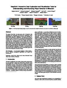
where am l are spherical harmonic coefficients determined via a spherical harmonic transformation, Ylm represent the spherical harmonics, and lmax is the order of truncation of the Laplace series. The most common way of representing HARDI data is the iconical representation, better known as glyphs. Each glyph corresponds to the local PDF on a sphere [20] or orientation distribution function (ODF) [27] calculated by the above mentioned techniques. The glyphs are given by the surface of the function graph {(r = ψ(θ , φ ), θ , φ ) | θ ∈ [0, π], φ ∈ [0, 2π]} defined on the spherical domain and plotted in radial direction. Recently, one can observe an increase in research activity regarding deterministic and probabilistic HARDI fiber tracking algorithms [4, 21, 13]. The resulting fiber visualizations give a clear representation of the data while a glyph visualization can be confusing and cluttered for the end user. However, all fiber tracking techniques exhibit several disadvantages, such as choice of initialization, sensitivity with respect to the estimated principal direction, lack of connectivity information between regions of the brain (deterministic), high computationally expense (probabilistic), and most importantly the lack of thorough validation which is needed before fiber tracking can be used in clinical applications. Knowledge about the local information is still quite important for testing and improving the fiber tracking techniques and, to the best of our knowledge, showing the local structure by glyph representation is the most common and reliable way of visualizing HARDI data. The traditional way of visualizing HARDI glyphs starts by generating a mesh of points on a sphere, and then deforming it according to Eq.1. This visualization is slow and memory consuming, especially if one wants to achieve smooth surfaces. For very smooth surfaces an icosahedral tessellation of 16th order is used, which generates 2256 points on a sphere. Thus, the visualization of a full brain slice and the interactive inspection of the data is practically impossible with this approach. Using a coarser mesh is an option to gain speed, but then lots of subtle details on the surface are missed and quite often the angular maxima are displaced, as is shown in Fig. 1. There are many HARDI related research questions where fast and reliable glyph visualization is useful. As mentioned, in the development of fiber tracking algorithms, it is useful to visualize the local information to validate whether the fiber tracks follow the underlying information. Because the signal-to-noise ratio can be low smoothing algorithms on the spherical function are of high importance, but these algorithms often have many parameters to tune. Being able to see the output in a fast manner can benefit the research in this area. In this paper we present a novel approach for fast detailed and accurate rendering of of high-dimensional diffusion-weighted (DW) data. After giving an overview of related work on HARDI visualization and GPU-based glyph rendering in section 2, we present the mathematical tools for visualizing spherical functions in section 3.

(a) order 2

(b) order 3

(c) order 4

(d) order 7

Figure 1: Traditional way of HARDI glyph visualization. The glyphs’ surface is getting smoother as the order of tessellation of the icosahedron is increased from order 2 (a) to order 7 (d). Changes of the maxima can be observed as the glyphs’ surface gets smoother.

In section 4 we show how to apply these tools to implement a GPUbased ray casting method for rendering HARDI glyphs. Analysis of the visual aspects and performance measurements follow in section 5. Finally, in section 6 we conclude this manuscript and address challenges in future work. 2

methods. This leads to more elaborate computations for the intersection of the view ray with the glyph and for the normal vector in this intersection. Using the properties of the spherical harmonics, we show how to solve these problems on the GPU in order to obtain a fast and accurate visualization of HARDI data that can be used in an interactive manner.

R ELATED W ORK

In DTI, glyphs are the basic tool to visualize the local structure. As mentioned in the previous section, the diffusion PDF is approximated by a second-order, symmetric, positive-definite tensor and therefore tensor glyphs are the most useful tool for representing the full tensor information. Commonly used shapes for visualizing the DTs are cuboids, ellipsoids and superquadrics [15]. There has been recent work in glyph packing algorithms by Kindlmann [16] and Hlawitschka [11], but these algorithms change the original grid positions of the local information for better visual perception. HARDI techniques overcome the disadvantages of DTI by applying high-order methods in the description of water molecule diffusion. However, these methods significantly raise the complexity of data processing and visualization. Among the available software packages for visualizing and processing HARDI data are Slicer [1] with the Qball plug-in [28] and Camino [3]. The latter one has very limited visualization capabilities since its core purpose is to process HARDI data. Recently, Shattuck et al. [23] developed a set of tools for visualizing ODF models. All of the mentioned packages apply the same concept. To obtain an ODF shape via polygons, they generate a mesh of points on a sphere and in or extrude these vertices. This approach renders an interactive scene only after the geometry is calculated. Furthermore, there is always a trade-off between the visual quality and rendering speed. The interaction is reported as 10 frames/sec on a single brain data slice with 225 samples on a sphere that approximates 4th order icosahedral tessellation. In their work, this limitation in rendering performance is being mentioned and GPU programming is suggested as a solution. A new and interesting work by Hlawitschka et al. [10] address the problem of improving the speed and robustness of the fiber tracking algorithms in HARDI. However, no performance information is given and the underlying field of high order tensors (HOT) or spherical harmonics (SH) representation still needs sampling on a predefined grid, which gives rise to the same disadvantages discussed above. Recent advances in capability and performance of GPUs have triggered several publications about the rendering of glyphs where ray casting on the GPU has been applied. Application areas include mathematics [7] and molecule rendering [24]. However, those methods focus on simple glyph shapes with few parameters, such as ellipsoids, where the intersection with the view ray can be computed analytically. Recently, Hlawitschka et al. [9] used GPU ray casting to render superquadric tensor glyphs [14]. The dimensionality of HARDI data, and thus the number of parameters that define the shape of our glyph is much higher than in the above mentioned

3

S PHERICAL H ARMONICS

FOR

HARDI

We being this section with a very brief introduction to spherical harmonics (SH) and describe how to compute properties that are needed for the ray-casting algorithm. In section 3.1 we explain why SHs are used and how to obtain real-valued SHs. Then, in section 3.2 we show how to compute an upper radial bound for the linear combination of SHs, which we will use later to generate bounding spheres for the ray-casting algorithm. Finally, in section 3.3 we show how to compute the normals of a spherical function needed in the surface shading of the glyph. 3.1

Spherical Harmonics

Spherical harmonics Ylm (θ , φ ) (SH) [17] form a complete orthogonal system for arbitrary spherical functions ψ(θ , φ ), which is expressed by the Laplace series ∞

ψ(θ , φ ) =

l

∑ ∑

m am l Yl (θ , φ ) .

(2)

l=0 m=−l

The expansion of spherical functions ψ(θ , φ ) via the Laplace series is practical, since spherical harmonics Ylm possess several beneficial properties. The most important property with respect to HARDI is the fact that SHs are part of the solution of the homogeneous diffusion equation ∂t p(r, θ , φ ,t) = κ ∆ p(r, θ , φ ,t) that governs the underlying physical process. Solving the diffusion equation via the separation of variables [22] with p(r, θ , φ ,t) = T (t)R(r)ψ(θ , φ ), one obtains for the angular part of the diffusion equation ∆S2 ψ(θ , φ ) = −l(l + 1) ψ(θ , φ ), with ∆S2 being the Laplace operator on a sphere S2 as defined in Eq. 3. Thus, the SHs are the eigenfunctions of this angular diffusion equation. ∆S2 Ylm (θ , φ )

 = =

1 1 ∂φ2 + ∂ sin θ ∂θ 2 sin θ θ sin θ −l(l + 1) Ylm (θ , φ ) .



Ylm (θ , φ ) (3)

Furthermore, one can view the Laplace series Eq. 2 as an inverse spherical Fourier transformation. As show in Eq. 3, the SHs are the Laplacian eigenfunction in spherical coordinates. On the other ~ ·~x hand, ei ω , cos (~ ω ·~x), and sin (~ ω ·~x) are Laplacian eigenfunctions in Cartesian coordinates. An expansion in these latter functions constitutes a Fourier transformation. Correspondingly, the SHs

form the basis functions of a spherical Fourier transformation, the spherical Fourier coefficients being am l . am l =

Z 2π Z π 0

0

ψ(θ , φ )Ylm (θ , φ ) sin θ dθ dφ .

(4)

The inverse spherical Fourier transformation is given by the Lapace series (see Eq. 2). The SHs are explicitly defined via associated Legendre polynomials Plm . s Ylm (θ , φ ) = ei m φ

2l + 1 (l − m)! m P (cos θ ) , 4π (l + m)! l

3.2

Bounding Sphere

For scaling and ray-casting purposes, it is necessary to have an upper bound for the maximum radius of the spherical function ψ(θ , φ ) represented by Laplace series in Eq. 7. From the Cauchy-Schwarz inequality, we know that 2



 ≤

∑ an bn

∑

n

a2n



∑

n

b2n

!2

N

if if if

m0

ψ(θ , φ ) ≈

lmax

l

∑

∑

˜m a˜m l Yl (θ , φ ) .

(7)

l=0,2,... m=−l

We truncate this Laplace series at a given lmax , since the angular sampling of a HARDI signal is finite as well, and due to the fact that noise becomes more dominant in higher frequencies. On the other hand, the higher the order lmax , the higher the angular frequencies that are captured, thus allowing more complicated and better resolved shapes for the reconstructed function ψ(θ , φ ). Hess et al. [8] proved, that order lmax = 4 results in good SNR performance and least angular error for the reconstruction of the correct orientation distribution function for HARDI data acquired in a clinical setup with b-values up to 4000s/mm2 . One can determine the spherical harmonic coefficients a˜m l via Eq. 4 or by any of the existing state-of-the-art HARDI techniques [5, 20, 19]. With small modifications the same approach can be applied to techniques like PASMRI [12], since the persistent angular structure exhibits functions similar to the orientation distribution function (ODF). Once we have pre-processed data i.e. volumes of spherical functions calculated by any of the above mentioned HARDI modeling techniques, we can reconstruct the angular PDFs or ODFs using the Eq. 7.

∑ a2n .

(9)

n=0

If we apply these inequalities to Eq. 7, we obtain for even l and lmax
2 ψ(θ , φ )

=

!2

lmax

l

∑

∑

˜m a˜m l Yl

(10)

l=0,2,... m=−l

 ≤ 

(6)



Re Ylm (θ , φ ) and Im Ylm (θ , φ ) represent the real and imaginary part of the Ylm (θ , φ ). These real-valued SHs Y˜lm (θ , φ ) are again or√ thonormal due to the normalization factor 2 and also eigenfunctions of the spherical Laplacian ∆S2 . Hence the previously stated properties of SHs remain valid. Only the tilde indicates the use of real-valued SHs. Employing basis functions of Eq. 6, the computation for preprocessing and rendering of the HARDI data is significantly simplified. Furthermore, note, that HARDI signals are real-valued and symmetric under inversion. It is therefore sufficient to expand a HARDI signal ψ(θ , φ ) by real-valued coefficients a˜m l and SHs Y˜lm (θ , φ ) with even l = 0, 2, 4, . . . lmax .

(8)

N

≤ (N + 1)

∑ an

n=0

 √
 2 Re Ylm (θ , φ ) Y˜lm (θ , φ ) = Y 0 (θ , φ )
 √l 2 Im Ylm (θ , φ )

, for an , bn ∈ R .

n

For bn = 1 this amounts to

(5)

with θ ∈ [0, π], φ ∈ [0, 2π] and integer indices l ≥ 0 and |m| ≤ l. The SHs as defined in Eq. 5 are complex-valued due to the factor ei m φ . Complex arithmetic is not established on GPUs, so that we have to rely on real-valued SHs. This is accomplished by the linear combinations of SHs Ylm and Yl−m to obtain 2 cos (m φ ) = (e−i m φ + ei m φ ) and 2 sin (m φ ) = (e−i m φ − ei m φ ). We adhere to the convention as in Descoteaux et al. [5] and define the real-valued SHs Y˜lm as



≤

lmax +1 2



lmax +1 2



lmax

!2

l

˜m a˜m l Yl

∑

∑

l=0,2,...

m=−l

lmax

l

!

l

2 (a˜m l )

∑

∑

l=0,2,...

m=−l

∑

!
2 Y˜lm

m=−l

With the SH identity [18] l

∑

Y˜lm


2

=

m=−l

2l +1 4π

(11)

we finally derive r |ψ(θ , φ )| ≤

v ul u max 1 lmax + 1 t ∑ 2 l=0

2l + 1 4π

l

∑

!
2 a˜m l

= rmax .

m=−l

(12) rmax can be used as the radius of an encompassing sphere that engulfs the glyph given by ψ(θ , φ ). This way we have a fairly good upper bound for the glyph size in the 3D volume of data voxels at hand. 3.3

Generating Normals

For proper shading it is essential to obtain the normals on the surface of the spherical functions ψ(θ , φ ). This is not a trivial task as these spherical functions consist of arbitrary, linear combinations of SHs. To resolve the problem we take a small detour and express the spherical function ψ(θ , φ ) by a volume density Φ(r, θ , φ ) in spherical coordinates. Φ(r, θ , φ ) := r − ψ(θ , φ ) .

(13)

Thus, the spherical function ψ(θ , φ ) constitutes the 0-contour of the volume density Φ(r, θ , φ ). Φ(r, θ , φ ) = 0. (14) r=ψ(θ ,φ )

This detour is feasible, because the gradient vectors of a density field are normal to its contours. Hence, ∇ Φ(r, θ , φ ) ⊥ ψ(θ , φ ) . (15) r=ψ(θ ,φ )

.

Furthermore, a gradient is a linear differential operator. So it is possible to pass it through the linear combination of SHs. lmax

∇ Φ(r, θ , φ ) = ∇ r −

l

˜m a˜m l ∇ Yl (θ , φ ) .

∑ ∑

(16)

l=0 m=−l

Obviously, we do not want to calculate the gradient field for all r, but only at the 0-contour with r = ψ(θ , φ ). We therefore take a look at the explicit expressions for the gradients ∇ r and ∇ Y˜lm (θ , φ ) to examine their r-dependence. Note, that the volume domain of Φ(r, θ , φ ) is parameterized by spherical coordinates. The gradient vectors below, however, are given in a Cartesian tangent space with x, y, and z-components.   cos(φ ) sin(θ )

∇ r =  sin(θ ) sin(φ )  .

(17)

cos(θ )

Apparently, ∇ r is r-independent so that a substitution r = ψ(θ , φ ) is not an issue. The gradient of a SH is given by   cos(θ ) cos(φ ) ∂θ −csc(θ ) sin(φ ) ∂φ 1 ∇ Y˜lm (θ , φ ) =  cos(φ ) csc(θ ) ∂φ +cos(θ ) sin(φ ) ∂θ  Y˜lm (θ , φ ) . r − sin(θ ) ∂

Figure 2: Illustration of our ray-casting algorithm.

θ

(18) Again, the SHs Y˜lm (θ , φ ) and also the vectorial differential operator in Eq. 18 are r-independent. Only a factor 1/r remains, which we can move outside the linear combination in Eq. 16. Hence, we can write ∇ Φ(r, θ , φ ) = ∇ r −

1 lmax l ˜m s ∑ ∑ a˜m l r ∇ Yl (θ , φ ) r l=0 m=−l

(19)

and obtain  ∇ Φ(r, θ , φ )

r=ψ(θ ,φ )

=



cos(φ ) sin(θ )  sin(θ ) sin(φ )  cos(θ )

−

(20)

  cos(θ ) cos(φ ) ∂θ −csc(θ ) sin(φ ) ∂φ lmax l 1 ∑ ∑ a˜ml  cos(φ ) csc(θ ) ∂φ +cos(θ ) sin(φ ) ∂θ  Y˜lm (θ , φ ) . ψ(θ , φ ) l=0 m=−l − sin(θ ) ∂ θ

After normalization, the gradients above are unit normals of the glyphs defined by the spherical function ψ(θ , φ ). 4 GPU-BASED R AY C ASTING OF S PHERICAL H ARMONICS Our goal is to show a set of glyphs to represent the spherical functions ψ(θ , φ ) in a cross-section of the data. This cross-section is defined by a plane-of-interest (POI) which the user can translate, rotate and resize using the mouse. The seed points that define the locations of the glyphs are implicitly given by the POI and a userspecified seed distance. When we render the scene, we step through all the seed points in order to deal with each glyph separately. Per glyph, the calculations are divided between CPU and GPU. On the CPU, we do the computations that can be done per glyph and on the GPU we run a ray casting algorithm per pixel. In the following sections we describe these calculations in more detail. 4.1 CPU On the CPU, we load the pre-computed spherical harmonics coefficients. Before rendering, we manipulate the coefficients according to parameters that the user can set interactively. The user can specify a scaling factor, with which all coefficients a˜m l are multiplied in order to change the size of the glyphs. Another user-defined parameter, the sharpness variable, determines a value by which a˜00 is

divided to reduce the influence of isotropic component Y˜00 and, thus, to enhance the anisotropic maxima of the glyphs. Finally, the user has the option to scale all glyphs independently to have the same a˜00 for each glyph, or to scale all glyphs by the same global maximum of a˜00 so that the differences in diffusion magnitude between different voxels becomes apparent. After manipulating the coefficients we need to render a geometry that covers the pixels in the viewport potentially occupied by the projection of the glyph. For this, we compute the maximum radius rmax of the spherical function as given in Eq. 12 and render an bounding cube that is aligned along the world axis and positioned with the glyph’s seed point as its center. The edges of the bounding cube have length 2 rmax . On the GPU we need rmax to compute bounds for the ray casting, so we pass its value as a vertex attribute. We also pass the 15 coefficients a˜m l as vertex attributes, since we truncate the Laplace series at order 4 for the reasons given in section 3.1. 4.2

GPU Algorithm Overview

In the vertex shader we only pass the coefficients a˜m l to the fragment shader and compute the view direction ~v by substracting the eye position V from the current vertex positions of the bounding box. Vector~v is automatically interpolated for use in the fragment shader, where we normalize it. Figure 2 illustrates the ray-casting process that is executed in the fragment shader. The three basic steps of our method are: 1. Compute the intersections of view-ray V with bounding sphere S which has radius rmax . If there are no intersections, discard the fragment. If there are intersections, we use them as bounds in the next step. 2. Approximate the intersection point I of V and the surface H defined by spherical function ψ(θ , φ ). 3. Compute the normal of H in I and do lighting calculations to compute the color of the current fragment. Update the Zbuffer using I. These three steps are discussed in detail in the following sections.

4.3

Intersection of View-Ray and Sphere

Before computing the intersection of the view ray V with surface H defined by ψ(θ , φ ), we compute the intersections of V with bounding sphere S . There are two reasons for this: 1. If there is no intersection of V with S , which can be determined very fast, the fragment can be discarded and we save the computations needed to determine intersection of V with H. 2. We use the intersections of V with S as bounds in the algorithm that determines the intersection of V with H . The intersections Inear , I f ar of V with S can be determined analytically by substituting the equation of the ray V (t) = V + t~v

(21)

into the equation of a sphere 2 (x − Px )2 + (y − Py )2 + (z − Pz )2 = rmax

Figure 3: Close-up of our GPU glyphs showing a detail of a synthetic phantom dataset of two crossing fiber bundles under an angle of 90 ◦

(22)

where P = (Px , Py , Pz ) is the center of the sphere and rmax the radius. The resulting equation can be solved using the quadratic formula. √ −b ± D µ= , where D = b2 − 4ac , (23) 2a with a

=

∑

~v2i ,

(24)

i∈{x,y,z}

b

=

∑

2(Vi − Pi )~vi ,

(25)

(Vi − Pi )2 − r2 .

(26)

i∈{x,y,z}

c

=

∑ i∈{x,y,z}

The number of solutions depends on the value of D. For D < 0 there is no intersection√and we discard the fragment. √ For D > 0, we have Inear = V ((b2 − D)/2a) and I f ar = V ((b2 + D)/2a). For D = 0, we obtain Inear = I f ar . 4.4

Intersection of view-ray and spherical function

Figure 2 shows a view ray V and how it can intersect a spherical surface S . In order to find the intersection of V and H , we start with a basic ray casting approach that does a linear search with discrete steps along V to find the first point on V that is inside H . For this, we initialize the point p on V with Inear and vector step to have the same orientation as ~v and user-definable length h. n = 0; while ((!IsInsideSH(p)) && (n < MaxN)) { p = p + step; n++; } MaxN is computed from the distance between Inear and I f ar and step-length h. If we reach n = MaxN before a point inside H is found, then there is no intersection and we discard the fragment. The boolean function IsInsideSH(p) is described below. The user can interactively change the value of h to ensure fast rendering and to make sure that h is not too large for important details to be missed. After the linear search, we initialize points upper, lower with p and p - step, which are on opposite sides of H , and use a binary search algorithm to refine the position of the intersection:

for (int i=0; i < NumRefineSteps; i++) { p = (lower + upper) / vec3(2.0); if (IsInsideSH(p)) upper = p; else lower = p; } p = (lower + upper) / vec3(2.0); In order to determine whether a point p is inside or outside H in IsInsideSH(p), we first compute p in local spherical coordinates for the current spherical function: d~

=

θ φ r

= = =

normalize(p − SHcenter) q 2 atan( dx + dy2 /dz ) atan(dy /dx ) length(p − SHcenter)

Now, if we compute ψ(θ , φ ) cf. Eq. 7 we get the radius of H in that direction. If r > ψ(θ , φ ) then p is outside H and if r < ψ(θ , φ ) then it is inside. For computing ψ(θ , φ ) we computed the analytical expressions for Ylm cf. Eq. 5 for l up to 4. 4.5 Normal Computation and Lighting We compute the normals in the intersection points on the ray-casted surface as described in section 3.3. In order to do this, we use Eq. 20 and the analytical expressions of the spherical harmonics. Using the normal, we use standard lighting according to the Phong lighting model. Furthermore, we use the commonly-used color coding in HARDI and DTI that maps the orientation vector that points from the center of the glyph to the surface, to a color, where red corresponds to mediolateral, green to anteroposterior, and blue to superoinferior orientation. The results are illustrated in Fig. 3. 5 R ESULTS In Fig. 4 we show a region-of-interest on a coronal slice of centrum semiovale since fibers of the corpus callosum (CC), corona radiata (CR), and superior longitudinal fasciculus (SLF) form a three-fold crossing there. This is a very interesting region, with known crossings and therefore it is very often a target for qualitative analysis of DW- MRI techniques. We generate artificial noiseless synthetic data of a 90 ◦ crossing according to Soderman et al. [25] (see Fig.

#glyphs 70 732 4125 4125 4125 4125

step size h 0.01 0.01 0.01 0.01 0.02 0.02

#refine steps 4 4 0 4 0 4

rendering performance (FPS) >100 70–90 10–23 8–23 ∼20 ∼20

Table 2: Rendering performance for our proposed GPU-based glyphrendering method with varying parameters.

3). We use this data to validate our implementation. The RGB color coding coincides with the orientation of the simulated volume. In the single fiber areas, we clearly observe the “peanut” shape representation of the ODF. The areas of crossings are correctly represented as well. In Fig. 3 we immediately observe the advantage of our GPU based rendering: the quality of the rendered glyphs is independent of the zooming factor. DW-MRI acquisition was performed on a healthy volunteer (25year old female) using a twice refocused spin-echo echo-planar imaging sequence on a Siemens Allegra 3T scanner (Siemens, Erlangen, Germany). The scanning was done using FOV 208 × 208 mm and voxel size 2.0 × 2.0 × 2.0 mm. Ten horizontal slices were positioned through the body of the corpus callosum and centrum semiovale. Data sets were acquired with 106 directions, each at b-values of 1000, 1500, 2000, 3000 s/mm2 . We visualize the data with our proposed technique and compare it with the previous methods that generate geometry via polygons. First, we analyze the visual results in 5.1 and then we give performance measurements in 5.2. 5.1

Visual Aspects

In Fig. 4(a) we show ODF glyphs rendered with the geometrybased method with 3rd order of tessellation of an icosahedron. A similar ROI is shown in Fig. 4(b). The increase of visual quality can be immediately observed, crossings become visually more clear, and there is an obvious 3D effect that perceptually helps in the distinction of the CC and CR structures 5.2

Performance

We compared the performance of the proposed method to the performance of the traditional method where geometry is generated. The results of the traditional and the proposed method are shown in table 1 and table 2 respectively. Rendering was done on a PC with an Intel Pentium 4 3.20 GHz CPU, 3 GB RAM and a GeForce 8800 GTX graphics card with 768 MB of memory. For the generation of geometry we used a custom VTK filter of which the output was rendered with a standard VTK polydata mapper. Although we did not optimize the methods that were used for generating and rendering geometry, the results clearly indicate that our proposed method outperforms the geometry-based method. Of course, in both methods the performance decreases when the number of glyphs increases. But the performance of the geometrybased method decreases drastically when the order of tessellation is increased. This poses a problem since the orders of tessellation that give good enough visual results cannot be rendered in an interactive way. Furthermore, with the geometry-based method it is impossible to interactively define the region-of-interest (ROI), because it needs to generate geometry for the glyphs in the new ROI. Also, when changing parameters such as scaling and sharpening, the geometry needs to be changed and thus this also cannot be done interactively. Our proposed method gives satisfactory visual results even with the lowest settings listed in table 2 (step size 0.02 and no refine steps). With these settings, the glyphs look smoother than with the

traditional method using 4th order of tessellation. Furthermore, we can define the current ROI interactively, since no geometry needs to be generated, and we can also change all rendering parameters interactively. For the figures 3 and 4b in this paper, we used the settings from the tables that give the best visual results, i.e. a step size h = 0.01 and 4 refinement steps. 6 C ONCLUSIONS AND F UTURE W ORK We presented a fast and flexible method for GPU rendering of HARDI glyphs. It is important to state that HARDI is an emerging area, exploding with new proposed techniques for data modeling, regularization, fiber tracking and more. Validation is still an open issue in HARDI. Showing the local information of the reconstructed PDF, ODF or any other function that resides on a sphere, in a fast way is essential for the development of the HARDI research. At the moment, to the best of our knowledge, there is no fast and interactive way for HARDI data exploration and visualization. Being able to interactively explore the quality of the obtained data, to detect the interesting areas for further inspection in a fast and reliable way, and to validate the new proposed fiber tracking techniques by supplying the local information will undoubtedly move the HARDI methods from pure research into clinically applicable new and better DW-MRI techniques for depicting the white matter structure of the brain. We stress that this visualization is aimed at researchers in the area of HARDI and not physicians, due to the complexity and cluttering of the data. This GPU-accelerated visualization will improve the working conditions of the researchers, allowing them smooth and interactive data exploration. The rendering technique is based on a spherical harmonic approximation of any function on a sphere. Therefore it is not method-specific. Any of the existing HARDI techniques that can be expressed by a SH basis or a high order tensor basis (there is a direct relationship between these two representations), can be used as a pre-processing step to the work with our algorithm. It will be useful to extend the method with specialized coloring and sharpening methods that will highlight maxima of a spherical function and possibly highlight inter-voxel coherence. We will also integrate the new method into our visualization tools for DTI so that we can visualize different imaging modalities together. In order to further increase the performance of the ray-casting method, we are investigating numerical methods such as Newton-Raphson for the computation of the intersection of the view ray with the surface represented by a spherical function. Finally, we will investigate computer graphics techniques such as deferred shading and make use of geometry shaders and vertex buffers to further improve the performance. ACKNOWLEDGEMENTS R EFERENCES [1] 3D slicer. http://www.slicer.org. [2] P. J. Basser, J. Mattiello, and D. Lebihan. MR diffusion tensor spectroscopy and imaging. Biophys. J., 66(1):259–267, January 1994. [3] P. Cook, Y. Bai, S. Nedjati-Gilani, K. Seunarine, M. Hall, G. Parker, and D. Alexander. Camino: Open-source diffusion-MRI reconstruction and processing. In 14th Scientific Meeting of the International Society for Magnetic Resonance in Medicine, 2006. [4] R. Deriche and M. Descoteaux. Splitting tracking through crossing fibers: Multidirectional q-ball tracking. In ISBI, pages 756–759. IEEE, 2007. [5] M. Descoteaux, E. Angelino, S. Fitzgibbons, and R. Deriche. Regularized, fast and robust analytical q-ball imaging. Magn. Reson. Med., 58:497–510, 2007. [6] L. R. Frank. Anisotropy in high angular resolution diffusion-weighted MRI. Magn Reson Med, 45(6):935–9, 2001. [7] S. Gumhold. Splatting illuminated ellipsoids with depth correction. In VMV, pages 245–252. Aka GmbH, 2003.

(a) Geometry-based

(b) GPU ray casting

Figure 4: ODF representations of the DW-MRI data with 106 gradient directions and b=2000 s/mm2 of a human subject in a ROI defined on a coronal slice in the centrum semiovale. The glyphs are shown for 4th order spherical harmonics, which are min-max normalized (a): Traditional way of HARDI glyphs rendering with 3rd order icosahedral tessellation so interaction is still possible. (b): Ray casting of the HARDI glyphs on GPU.

#glyphs 70 70 70 700 700 700 4125

tessellation order 3 4 7 3 4 5 4

#points per glyph 168 252 642 168 252 362 252

generation time (s)