Digitization and Image CaptureâSampling. Keywords: Sampling, Tile-Based Methods, Blue-Noise Distribu- tion, General-Noise Distribution, Fourier Spectrum.
To appear in TOG 33(4) SIGGRAPH 2014
Fast Tile-Based Adaptive Sampling with User-Specified Fourier Spectra Florent Wachtel1 Adrien Pilleboue1 David Coeurjolly2 Katherine Breeden3 Gurprit Singh1 1 4 4 Ga¨el Cathelin Fernando de Goes Mathieu Desbrun Victor Ostromoukhov1,2 1
Universit´e de Lyon
2
CNRS-LIRIS
3
Stanford University
4
Caltech
Precomputation
Subdivision rules
Tiling
Centroids
Runtime
Optimized centroids
Sampling
Figure 1: Using a carefully-designed set of subdivision rules, our approach constructs a self-similar, equi-area tiling that provides an even, unstructured distribution of tile centroids. Per-tile sampling points are then generated through offline optimization of the tile centroids in a series of local patches using any existing point set optimizer; the resulting offsets between original and optimized point locations are stored in a lookup table. These offset vectors are finally used at runtime to convert tile centroids into point set distributions with spectral properties closely matching those of the optimizer, but several orders of magnitude faster than current spectrum-controlled sampling methods.
Abstract We introduce a fast tile-based method for adaptive two-dimensional sampling with user-specified spectral properties. At the core of our approach is a deterministic, hierarchical construction of self-similar, equi-area, tri-hex tiles whose centroids have a spatial distribution free of spurious spectral peaks. A lookup table of sample points, computed offline using any existing point set optimizer to shape the samples’ Fourier spectrum, is then used to populate the tiles. The result is a linear-time, adaptive, and high-quality sampling of arbitrary density functions that conforms to the desired spectral distribution, achieving a speed improvement of several orders of magnitude over current spectrum-controlled sampling methods. CR Categories: I.4.1 [Image Processing and Computer Vision]: Digitization and Image Capture—Sampling. Keywords: Sampling, Tile-Based Methods, Blue-Noise Distribution, General-Noise Distribution, Fourier Spectrum Links:
1
DL
PDF
W EB
Introduction
Sampling is key in a variety of graphics applications. In rendering, for instance, point sampling of continuous functions at strategically chosen locations allows for the accurate evaluation of spatial integrals. The spectral properties of these point samples have long been
understood to be crucial in defining the notions of bias (systematic deviation from the ground truth), variance (signal-to-noise ratio), and aliasing (appearance of undesirable artifacts) in sampling-based evaluations. In particular, blue noise point sets [Ulichney 1988] are widely regarded as excellent due to their particular spectrum [Pharr and Humphreys 2010]. Recent work has made more explicit the relationships between spectral content of a signal, spectral properties of sampling points, and resulting bias, variance, or aliasing [Durand 2011; Subr and Kautz 2013]. Consequently, exercising precise control over the spectral properties of sampling points has been a recent subject of ¨ research [Zhou et al. 2012; Oztireli and Gross 2012; Heck et al. 2013]. Unfortunately, current algorithms offering spectral control are prohibitively slow—and thus poorly suited for what is arguably their most important application: Monte Carlo or Quasi-Monte Carlo integration. The only methods able to achieve the high throughput of blue noise sample points commonly needed in practical applications are based on precomputed tiles [Lagae et al. 2008]. However, despite heavy offline optimizations, tile-based methods always exhibit spurious peaks and deficiencies in their associated Fourier spectra. These artifacts may be very pronounced if the tile barycenter is used as the sole sample per tile (Fig. 2), and remain visible even when there are multiple optimized samples per tile (Fig. 13) due to inherent patterns in the shape and positioning of the tiles. We present an efficient tile-based sampling system capable of generating high quality point distributions with controllable spectral properties at a rate of several millions of samples per second on commodity hardware—several order of magnitudes faster than current spectrum-controlled sampling methods. In sharp contrast to previous work, our approach relies on a deterministic set of production rules to produce self-similar, equi-area tiles whose centroids generate a blue noise distribution free of spurious spectral peaks. This tiling serves as a foundation for a lookup table based sampling system, in which the optimal positions of sampling points within each tile are determined by an offline optimization process to conform to a user-defined spectrum. Our approach thus allows for linear-time adaptive sampling of arbitrary density functions with precise spectral control over the resulting distributions. Contributions.
DC 0 .9 0 .8 0 .7 0 .6 0 .5 0 .4 0 .3 0 .2 0 .1 0 .0
(a)
(b)
(c)
(d)
(e)
(f)
Figure 2: Spectral characteristics of various tile-based sampling methods for one sample point per tile. Top row: tiling and tile centroids. Bottom row: Fourier spectra of tile centroids. Circles on the right portion of each spectrum indicate peaks of size 0.1 and greater (DC value of 1). Left to right: (a) Penrose tiles, (b) polyominoes, (c) regular hexagons, (d) irregular hextiles h˜ (Sec. 2.2), (e) regular trihexes t (Sec. 3.1), (f) irregular trihexes ˜ t (Sec. 3). The spectrum of irregular trihexes ˜t is further improved via the optimization method described in Sec. 4.
1.1
Related work
In order to motivate and highlight our contributions, we briefly review the main approaches to generating point distributions with known desirable sampling properties and a few representative works that illustrate them best. A first series of algorithms were formulated in the 1980s to eliminate aliasing artifacts in ray tracing [Dipp´e and Wold 1985; Cook 1986; Mitchell 1991]. In particular, jittered sampling achieved a linear complexity compromise between uniform and fully-stochastic sampling. Poisson-disk distributions were also introduced via dart throwing [Cook 1986], with many improvements and extensions proposed [McCool and Fiume 1992; Ebeida et al. 2011]. Current GPU implementations of stochastic sampling can generate over 100K samples per second [Wei 2008; Ebeida et al. 2011]. However, stochastic sampling methods such as jittering or Poisson-disk sampling produce distributions with relatively high variance by today’s standards, and do not offer spectral control. Stochastic sampling.
Over the last few years, higher quality sampling techniques have been proposed in which sample positions are spatially optimized to produce blue noise distributions [Balzer et al. 2009; Chen et al. 2012; Schmaltz et al. 2010; Schl¨omer et al. 2011; Fattal 2011; de Goes et al. 2012]. While these methods generally produce high-grade isotropic sampling, in practice their running times are prohibitive for large point sets. Recent methods [Zhou ¨ et al. 2012; Oztireli and Gross 2012; Heck et al. 2013] have added control over the Fourier spectra of sample points by optimizing over a differential domain, an intermediate space between the spatial and Fourier domains [Wei and Wang 2011]. Once again, these new methods suffer from prohibitive running times due to the need to iteratively proceed through inherently local optimizations. Optimal sampling.
furthered this work, resulting in fast and adaptive sampling of variable density functions. However, Wang-tile approaches all suffer serious drawbacks: the low count of prototiles and their placement on a square lattice induce a grid of peaks in the spectral domain, thus leading to sampling artifacts. A typical implementation of Wang tiles uses thousands of points per tile to alleviate these spectral peaks, at the cost of a significant increase in memory. Additionally, these methods rely on ranking the sampling points within each tile, bringing forth another critical flaw: for densities that are not a power of the subdivision factor, partial filling of prototiles is driven by a ranking algorithm [Ulichney 1993], not through offline optimization. This issue is clearly visible in the second row of Figure 11. Penrose tiles [Ostromoukhov et al. 2004] and polyominoes [Ostromoukhov 2007] were proposed in lieu of Wang tiles as a convenient alternative. With one sample per tile, these techniques allow for finer adaptivity when dealing with steep density functions. However, single-sample tiles result in rather poor Fourier spectra, as they exacerbate the presence of tiling structures which are overly simple or regular. While many other regular, semi-regular, or even irregular tilings may provide some improvement – likely at the price of implementation complexity – we are not aware of any self-similar tiling that fulfills the need for isotropic and even distributions.
1.2
Our Approach at a Glance
While existing tiling methods offer the best compromise between speed and quality of sampling, they fail to satisfy the two competing properties of using a deterministic, hierarchical construction, while generating a high quality isotropic, even, and non-periodic distribution of tiles. In this paper, such a novel tiling based sampling method is introduced. At its heart is an adaptive non-periodic tiling with equi-area tiles, paired with an offline computation of a table of optimized (spectrally-controlled) point sets defined over the tiles. From multiple failed attempts at improving previous tiling methods, we derived a few key insights that guided us in the design of our novel approach. First, we selected hexagons as the building blocks of our tiling rather than the squares used in Wang tiles [Cohen et al. 2003] and polyominoes [Ostromoukhov 2007]; hexagons offer an additional symmetry axis, better intrinsic spectral properties, and only one adjacency relationship between neighboring blocks [Gr¨unbaum and Shephard 1986]. Rationale for our choice of tiling.
A decade ago, Cohen et al. [2003] proposed a sampling method relying on the offline placement of samples within repeated tiles. Their approach was based on Wang tiles [1965] containing precomputed Poisson disk distributions, and was able to produce point sets containing desirable spectral properties with unmatched efficiency. Recursive tile subdivision [Kopf et al. 2006] and an improved management of tile borders [Lagae and Dutr´e 2006] Tile-based sampling.
Second, we derived a hierarchical and deterministic subdivision process based on trihexes (i.e., connected agglomerates of three hexagons, Fig. 2(e)) as prototiles to break the symmetries of the regular hexagonal lattice—much like polyominoes were unions of squares introduced to create more complex tiling structures on a square lattice. Finally, we devised a hierarchical, deterministic, and area-preserving border shuffling procedure that mimics a stochastic process in order to remove remaining frequency peaks in the resulting Fourier spectrum (Fig. 2(f)). We combine these three crucial features to create non-overlapping tiles whose barycenters form a high quality blue noise distribution. Note that each component is necessary: for instance, border shuffling without trihex subdivision only partially improves the spectrum of a tiling (Fig. 2(d)).
As hinted by the subtle anisotropic structure visible in Fig 2(f), the removal of spectral peaks through our novel tiling may not be sufficient for most sampling purposes. Equipped with a non-periodic and even distribution, we describe the construction of lookup tables that associate each tile with an optimized point location, removing residual anisotropy and allowing for the efficient generation of high quality samplings at runtime. Existing optimization procedures may be used in this offline step to generate samplings with given spectral properties. Point sets are stored as offsets from the centroid of each polyhex and are made coherent across subdivision levels, thus guaranteeing high quality adaptive sampling of arbitrary density functions. From tiles to controllable sampling.
H
Throughout this paper, we will denote by the regular hexagonal lattice and a scaled down version of this lattice. Hexagons Hi ∈ are subdivided into quasi-hexagonal tiles hi we call hextiles, formed by the union of λ smaller hexagons from . Here, λ is a centered hexagonal number Cn , with Cn := 1, 7, 19, 37, 61, ... for n = 1, 2, 3, 4, ... [Conway and Guy 1996]; while we adopt λ := C4 = 37 to minimize memory requirements and complexity, other Cn can be used as subdivision factors (Appendix C). The partition formed by these hextiles is denoted as H. Hextiles are further made irregular by randomly reassigning small hexagons on to adjacent hextiles while preserving each hextile’s e of irregular hextiles connectedness and area, creating a tiling H {h˜ i }. We use trihexes (i.e., connected agglomerates ti of three hexagons) as prototiles, such that irregular trihexes (i.e., connected agglomerates ˜ t i of three irregular hextiles) will form the 407 tiles, unique up to rotations and translations, of our final tiling T (Sect. 3.2). Table 1 illustrates our notations used throughout this paper. Notation.
H
h
h
1.3
We present our approach in four parts. Section 2 describes the creation of an irregular, equi-area tiling with hexagonal topology through border shuffling. Section 3 then introduces our trihex-based tiling, an extension of Ostromoukhov’s polyominoes [2007], which, when used in conjunction with irregular hextiles, generates our tiling structure. The tiles’ centroids will be shown to form a blue noise distribution free of spectral artifacts. We detail in Section 4 an adaptive sampling system with spectral control through an offline optimization of sample points on tiles. We finally demonstrate in Section 5 that our approach generates sampling points as fast as previous tile-based methods, but with state-of-the-art quality Fourier spectra on par with the best existing optimization methods.
2
Description
See also
Hi
Regular hexagon from regular grid
H.
Sec. 2.1, Fig. 3
hi
Hextile; partition of (smaller regular grid) into hextiles is denoted H.
Sec. 2.1, Fig. 3
h˜ i
Irregular hextile; partition of e. irregular hextiles is denoted H
ti
Regular trihex on
˜ ti
Irregular trihex; partition of into irregular trihexes forms tiling T .
h
h into
H.
Sec. 2.2, Fig. 4 Sec. 3.1, Fig. 5
h
Sec. 3.2, Fig. 8
Table 1: Main notations used in the description of our approach.
Generating Irregular Hextiles
We begin with the construction of a hierarchical tilling in which each tile is an equi-area quasi-hexagon with randomized borders.
2.1
Quasi-Hexagonal Tiling
H
From the regular hexagonal lattice (Fig. 3(a)) we create quasihexagonal regions we call hextiles, composed of λ hexagons from a finer regular hexagonal grid (Fig. 3(b)): each hexagon Hi ∈ is thus mapped to a hextile hi retaining the hexagonal structure of elements of in that it still has six neighboring tiles. These hextiles form a tiling H of the plane and an equi-area partition of . This construction defines a subdivision from (spanned by the directions ~ 1 and U ~ 2 ) to H (spanned by ~u1 and ~u2 ) whose subdivision factor U is λ—chosen to be 37 to offer sufficient granularity (Appendix C). This subdivision can be recursively repeated down to any level.
h
H
H
h
H
H
H
hi
hj Hj
~2 U
h
Notation
Outline
Hi
~u1
Hk
~1 U
hk
~u2
(a)
(b)
Figure 3: Quasi-hexagonal tiles. (a) The unbounded, regular hexag~ 1, U ~ 2 ). (b) The unbounded, quasional lattice generated by (U hexagonal lattice H over the finer regular hexagonal lattice and generated by (~u1 , ~u2 ). Each regular hexagon Hi in corresponds, through subdivision, to a hextile hi made up of λ small hexagons.
H
2.2
h
H
Border Shuffling
H
Due to its regular structure, and its subdivisions induce major spectral artifacts when used for sampling (Fig. 2(c)). To disrupt this structure, we introduce irregularity in the hextile borders while maintaining both the area and topology of the original hextiles {hi }, resulting in irregular hextiles {h˜ i } that form, by construction, a e of the plane. tiling H We modify tile geometry using a stochastic process that reassigns hexagons of along the original border from one hextile to an abutting one, thus maintaining the tiling property of the resulting irregular hextiles. To encode this border alteration, we use one bit per boundary hexagon to indicate if it is kept as is or Discrete border alteration.
h
✁ ✁ ✁
reassigned to the adjacent hextile. One cannot pick random bits to alter shape: this would likely affect the evenness of the tiling by creating islands or holes, or by changing the tile area. Therefore, border bits must be carefully selected to guarantee the validity of the final irregular hextiling. A simple charac- a h terization of valid border bits is achieved a by considering triplets of connected border a c c a c c tiles. For each, we associate a triplet of binary h b words A := a0 a1 a2 a3 , B := b0 b1 b2 b3 , and b C := c0 c1 c2 c3 called a triple-edge modifier b h using the convention depicted in the inset figb ure, where 0 indicates no local reassignment. As discussed in Appendix A, each triple-edge modifier must consist of three words A, B, and C containing an equal number of nonzero entries, none of which terminates in the sequence “01.” Note that this straightforward characterization of valid triple-edge modifiers is in fact sufficient for any λ. Triple-edge modifiers.
3
i
2
1
0
0
j
1
2
3.1
Hierarchical Trihex Tiling
We adapt the polyomino tiling construction from [Ostromoukhov 2007] to our hexagon-based approach, first without border shuffling. Unlike the original square-based method, we use prototiles that are m-polyhexes, i.e., connected conglomerates of equal numbers of hexagons [Gr¨unbaum and Shephard 1986]. While an arbitrary value of m might be used, we choose m = 3 (i.e., trihexes) as it minimizes the memory requirement for our lookup tables while achieving our goal of improving spectral properties (Appendix C).
3
Prototiles
0
Subdivision Rules ✄ ☎ ✄
1
2
✁
✆
✂
k
3
t (a)
a0 c 0 c 1 c 2 c 3 b 2 a3 1 0 0 0 1 0 0 a2 a3 b 3 b0 1 0 0 0 a1 a2 b1 0 0 1 a0 c 0 c 1 c 2 c 3 b 2 a1 0 0 1 1 0 0 0 a0 c 0 c 1 a3 b 3 b0 1 0 1 h˜ i hi 0 0 0 a2 b1 b0 0 0 1 a1 c 0 c 1 c 2 c 3 b2 b1 0 0 0 0 1 0 0 a0 c 0 c 1 c 2 c 3 b 2 a3 b 3 h˜ j hj 1 1 0 0 0 1 0 0 a2 a3 b 3 b0 0 0 0 0 a2 a1 b1 1 1 1 a0 c 0 c 1 c 2 c 3 b 2 a1 0 0 1 0 0 0 1 ˜ a0 c 0 c 1 c 2 a3 b 3 hk hk b0 0 1 0 1 0 0 0 a2 b0 b1 0 0 0 a1 c1 c2 c3 b2 b1 0 0 0 1 1 1 a0 c 0 c 1 c 2 c 3 b 2 a3 b 3 0 0 0 1 0 1 0 0 a2 a3 b 3 b0 1 0 0 0
(a)
(b)
Figure 4: Effect of edge modifiers. From a set of hextiles hi and e is random valid edge modifiers (a), a set of irregular tiles h˜ i in H obtained (b) which maintains the topology of the initial tiling as well as each tile’s initial area.
2.3
Irregular Hextiling
Given the choice of λ = 37, there is a total of 120 valid tripleedge modifiers, forming a sufficiently large set for our shuffling e , we begin with the purposes. To construct an irregular tiling H regular tiling H and assign three independent triple-edge modifiers to each hextile as shown in Fig. 4(a). Reassigments are made based on the binary words bordering each regular tile hi , resulting in irregular tiles h˜ i that are, by construction, also comprised of λ hexagons from (Fig. 4(b)). This irregular hextile is guaranteed to be homeomorphic to a disk (Appendix A). Thanks to this areapreserving border shuffling, our subdivision process from to e , with the same H can thus be modified to instead map to H subdivision factor λ.
h
H
3
H
Trihex-based Tiling via Irregular Hextiles
Once the border shuffling procedure is applied, the resulting tiling e will contain a rich set of irregular hextiles. While improved, its H underlying quasi-hexagonal structure still results in an unsatisfactory distribution of tile centroids (Fig. 2(d)). This issue is addressed next through the use of m-polyhex tiles (here with m = 3, see Appendix C), extending the polyominoes method [Ostromoukhov 2007] to our irregular hextiling setup. The resulting construction of subdivision rules based on irregular trihexes will serve as the basis of the tiling T used in our sampling approach.
T (b)
✝ ✝
H
Figure 5: (a) 11 configurations of trihexes on . (b) The library of subdivision rules {t → T}, where the quasi-trihex tile associated with t after subdivision is partitioned into a set of λ = 37 trihexes. There are 11 trihex prototiles up to symmetries, shown in Fig. 5(a). Moreover, we can extend the decomposition from to H defined in Section 2.1 to trihexes: for each triplet of hexagons of forming a prototile, we can trivially create a “quasi-trihex” on , i.e., a group of three hextiles shaped like the original trihex (see Fig. 5(b)). In order to create a full hierarchical tiling, we decompose each quasi-trihex tile into a set of λ trihexes. This decomposition is performed offline using a simple discrete optimization as described in Appendix B. The result is a cache of 11 subdivision rules {ti → Ti } transforming trihexes in to λ trihexes on , as illustrated in Fig. 5(b). This hierarchical tiling system is non-periodic, as follows from Statement 10.1.1 in [Gr¨unbaum and Shephard 1986].
H H h
H
h
As substantiated by Fig. 2(e), these trihex subdivision rules {ti → Ti } form a tiling with a distribution of centroids whose Fourier spectrum has much reduced peaks when compared to the original spectrum of H. To further scramble this distribution, we now incorporate border shuffling.
3.2
Irregular Trihex-based Tiling
In order to mimic an ergodic stochastic process, border shuffling might be added at each level of the subdivision. However, this would defeat the purpose of using tiles for fast sampling, as it would create an exponentially large number of tiles. We thus must use our irregular tiling from Section 2 parsimoniously, adding just enough irregularity to the tiles without requiring undue computational and memory overhead. We achieve this balance by constructing a larger, but limited, number of subdivision rules. We first limit the number of irregular hextiles in our tiling process through bi-periodicity in our triple-edge modifiers. We choose two generative integer vectors g~1 = 7 · ~u1 −4 · ~u2 and g~2 = 4 · ~u1 +3 · ~u2 , where ~u1 and ~u2 are the vectors spanning our hextiling (see Fig. 3), such that the area A of the parallelogram formed by these two vectors is A(g~1 , g~2 ) = λ · Ahex , where Ahex is the area of each hextile h˜ 1 . The fundamental region of this bi-periodic construction is highlighted in Fig. 6 Limited Irregularity via Bi-Periodicity
1 More
generally, if λ is the nth centered hexagonal number, these vectors are chosen to be g~1 = (2n+1) · ~ u1−(n+1) · ~u2 and g~2 = (n+1) · ~u1+n · ~u2 .
Irregular Trihexes
Subdivision Rules ✄ ☎ ✄ ✁
✆
✂
g~2 e H
h˜i ~ u2
g~1
~ u1
t˜ (a)
Figure 6: Periodic tiling based on two integer basis vectors g~1 and e of λ irregular hextiles {h˜ i } (highlighted). g~2 , creating a small set H We then constrain our triple-edge modifiers to reflect the periodicity generated by these two vectors. Consequently, we must create a e repeated set of only λ different irregular hextiles {h˜ i }i=1..λ := H e , as illustrated in Fig. 6. Notice that, by construction, we over H e based on the can naturally enumerate these irregular hextiles in H (arbitrary) enumeration of the λ hexagons in produced when subdividing a hexagon from (see Fig. 3): one can therefore assign a hex-index ∈ [1..λ] per irregular hextile, uniquely determining the indices of the corresponding 6 adjacent hextiles. An example of this enumeration is given in Fig. 7.
h
H
Each irregular hextile is further e subdivided into smaller irregular hextiles from the limited set H: starting from an irregular tile h˜ i with hex-indexed hexagons in , we first apply one regular subdivision step. Then, if a hexagon h has hex-index i, the irregular tile used to replace h will be the e This subdivision step is illustrated in ith irregular hextile in H. Fig. 7. The consistency of the subdivision system—in particular, the property that the irregular hextiles in Fig. 7 (right) do not overlap—is e coincide with the indices used in the due to the fact that indices in H → H subdivision step. Subdividing Irregular Hextiles.
h
H
✂
✟ ✁✞
✝ ✄ ✁✂ ✁
✆ ✁☎
✂
✁✟
✞✂ ✁
✂
✁✁
✞✞
✞
✁
✁✠ ✟
✞☎
✁ ✞
✞✝
☎
✌☞ ☛✏ ✌☛ ✒ ✡☞ ✌✡ ✒ ✌✓ ✌✑ ✏ ☛☞ ✡☛ ✡✡ ✌✌ ✌✓ ✌✑ ✡✓ ✡✑ ✌✎ ✌✍ ☛☛ ☛✡ ✡✌ ✡✓ ✡✑ ☛✓ ☛✑ ✡✎ ✡✍ ☛ ✡ ☛✌ ☛✓ ☛✑ ✌ ✓ ☛✎ ✡✒ ✓ ✌☞ ✌☛ ✑ ✎ ☛✍ ☛✒ ✡✏ ✌☞ ✌☛ ✡☞ ✡☛ ✌✡ ✌✌ ✍ ✒ ☛✏ ✡☞ ✡✡ ✡✌ ✌✓ ✌✑ ✏ ✡✓
✞ ✠
✞✟
✄ ✁✂
✁ ✄
✞✠
✆
✁✝
✁
✝
✁☎
✁✟
✂
✁✁
✞✞
✞
✁
✁✠ ✟
✞☎
✁ ✞
✞✝
☎ ✞✂
✁
✟ ✁✞
✆
✂
✞✄ ✠
✂
✓ ☛✏ ✌☛ ✒ ✡☞ ✌✡ ✌✓ ✌✑ ✏ ☛☞ ✡☛ ✡✡ ✌✌ ✌✓ ✌✑ ✡✓ ✌✎ ☛☛ ✡✌ ✡✓ ☛✌ ☛✓ ✡✑ ✡✎ ✌✍ ☛ ☛✡ ☛✌ ☛✓ ✡✑ ✌ ✓ ☛✑ ☛✎ ✡✍ ✡✒ ✡ ✌ ✓ ☛✑ ✑ ☛✍ ✡✏ ✌☛ ✎ ☛✒ ✌☞ ✌☛ ✡☞ ✡☛ ✌✡ ✌✌ ✍ ✒ ☛✏ ✡☞ ✡✡ ✡✌ ✌✓ ✌✑ ✏ ✡✓
✞ ✠
✞✟
✄ ✁ ✄
✞✠
✆
✁✂ ✁✝
✁
✝
✁☎
✁✟ ☎
✞✂ ✁
✞✞
✞
✁
✁✠ ✟
✞☎
✁✁
✞ ✞✝
✞ ✠
✞✟
✂
✁ ✄
✞✠
✆
✁✝
✞✄ ✠
Figure 7: From an irregular hextile h˜ i with indexed hexagons (left), we apply one regular subdivision step to construct sub-hextiles hi (center). Replacing each of these λ sub-hextiles with a different e creates a seamlessly subdivided irregular irregular hextile from H hextile (right). Since there are λ irregular hextiles in e and 11 configurations of classical trihexes in , there may be H 11 · λ = 407 different trihexes in T (see, e.g., Figs. 8(a) and 10). We construct our final tiling, at any level of refinement, as follows. First, we make random selections of admissible edge modifiers to construct e and compute the set Te of all irregular trihexes (|Te | = 11 · λ). For H e to each irregular trihex ˜ t ∈ Te , we use a subdivision from to H generate finer structure. Such finer structure on the subdivided grid is decomposed into a collection of λ trihexes of irregular hextiles, e is denoted T in Fig. 8(b). Finally, the subdivision rule ˜ t →T recorded. As mentioned in Section 3.1, we discuss the technique used to perform this decomposition into trihexes in Appendix B. The resulting trihex tiling induced by the library of subdivision rules e is non-periodic, just as in the irregular hextile case. {˜ t → T} Full Subdivision Process.
H
H
(b)
Finally, trihexes in T are indexed by a rank (i.e., an integer in {1 . . . λ}). This choice of ordering is crucial to obtaining maximal quality during the adaptive sampling described in Section 4.3, as it assigns indices such that sequentially ranked trihexes are as physically distant from each other as possible— thus offering, between subdivision levels, a generalized Halton-like sequence of tile barycenters. We use the classical void-and-cluster method [Ulichney 1993; Kopf et al. 2006; Ostromoukhov 2007] to e of the irregular trihex ˜ t 0 in each find the ranking rank (˜ t 0 |˜t → T) e ˜ subdivision rule t → T. Rankings within the subdivision of a few trihexes can be seen in Fig. 10. Ordering of Sub-Trihexes.
3.3
Concise Structural Indices
In order to efficiently access trihex lookup tables during sampling, we must be able to uniquely, yet concisely, identify a given tile at an arbitrary subdivision level. We address this important implementation issue by using hybrid structural indices as follows. In our tiling T , an irregular trihex ˜ t k at subdivision level k could be uniquely defined by a sequence of subdivision rules from the library, i.e., as a sequence of trihex ranks2 : e 1 ) ⊕ . . . ⊕ rank (˜ ek ) , rank (˜ t 1 |˜t 0 → T t k |˜t k−1 → T
✁
✟ ✞ ✝ ✝
Figure 8: (a) Examples of irregular trihexes in T (only 11 out of e for 11 · λ are shown). (b) The library of subdivision rules {˜ t → T} all irregular trihexes.
✟ ✁✞
✆
✂
✞✄ ✠
✂
e T
(1)
e i . However, in order to support adaptive with ˜ t i a trihex in the set T sampling (and thus, deep subdivision), k might become arbitrarily large, making trihex identifiers intractable in practice. We thus desire to formulate structural indices that are: • finite, but from which trihexes of arbitrary resolution can be represented; • such that trihexes with the same structural index will share the same local configuration of trihexes, regardless of their subdivision level These properties can be achieved by exploiting the cyclic structure in the sequence of trihex ranks, which leads to a limited number of possible local tile neighborhoods. In fact, we propose to use as structural indices a mix of neighborhood indices and ranks, thus offering a balance between the tile indexing proposed in [Ostromoukhov et al. 2004] (ranks only) and [Ostromoukhov 2007] (neighborhood indices only). Instead of explicitly representing the entire subdivision path from ˜ t0 to ˜ t k , we characterize ˜t k by the rank of its last l subdivision steps e k , and replace the prepending path from t0 to ˜ ˜ t k−l → T t k−l with a neighborhood index based on the trihexes surrounding ˜ t k−l , which we denote n(˜ t k−l ). ek ) . id(˜ t k ) := n(˜t k−l ) ⊕ rank (˜t k |˜t k−l → T 2 If
(2)
ranks are integer numbers on b bits, ⊕ is the concatenation operator on bits. The trihex identifier would thus require k · b bits.
We found that using l = 1 provides a good balance between quality and lookup table size (see Appendix C). The neighborhood index n(˜ t ) for a given irregular trihex ˜t is a unique number representing the trihex adjacency around ˜ t , see Fig. 9. Such indices are computed from a local analysis of irregular trihex adjacencies in the subdivision rules: we observe that for each ˜ t , the number of unique neighboring trihex configurations n(˜ t ) is 336 on average. An irregular trihex index is thus defined as one rank (a number between 1 and λ) and one neighboring index, which in our actual implementation leads to about 5M possible indices–thus 23 bits, however deep one needs to subdivide the tiles.
Figure 9: Neighborhood of a trihex. Two trihexes (dark blue) with identical neighborhood indices have the same 1-ring of neighboring trihexes (light blue) but may have different (n > 1)-rings. Point-set optimizations start with the centroid of each tile and are averaged over all possible configurations of a trihex’s vicinity (dotted circle).
4
Adaptive Tile-based Sampling
At any subdivision level k, our tiling method generates an artifactfree blue noise distribution of trihex centroids with constant spatial sample density (Fig. 2(f )). However, single-sample-per-tile approaches produce high quality results only for powers-of-λ densities: in between two levels of subdivision, the spectral properties of the centroids’ distribution are dictated solely by the ranking algorithm, resulting in suboptimal sampling. In order to remediate this issue and offer control over the distribution spectrum for the sampling of arbitrary constant densities, we now show how to generate spatiallyoptimized point samples for each tile in an offline stage, leading to high-quality adaptive sampling at runtime.
4.1
Lookup Sampling Table
We first construct a lookup table D to exert control over the spectra at intermediate levels of subdivision: for each tile, we will compute a set of optimized point samples at each range of ranks Rr := [0 . . . r] (with r < λ), where sample locations are stored as offsets from the tile centroid. More precisely, we begin with a trihex for each neighborhood index and subdivide it several times, generating a large patch containing about N trihexes (the value of N is optimizer dependent; see Sec. 4.2). Inside each patch, each trihex ˜ t is subdivided once more, creating λ sub-trihexes. For each range of ranks Rr and for each trihex with structural index id in this patch, we create a point set containing the barycenter of the id trihex along with the N nearest sub-trihex barycenters with ranks in Rr (see Fig. 10). These points are then spatially optimized using any existing optimizer to improve their spectral distribution (discussed below). Finally, the resulting point set is converted into offsets from the barycenter of the id trihex, which are then stored in the lookup table entry D[r, id] for rank range Rr and structural index id. Note that our initial trihex subdivisions are such that we will run multiple optimizations of the same structural index. However, our construction of structural
(a) R1
(b) R2
(c) R3
(d) R37
Figure 10: Optimization snapshots for various sample densities (i.e., various rank ranges Rr ). Black dots mark the centroids of sub-tiles (colored); arrows indicate the sampling offsets computed in the first iteration of the optimization loop.
indices is such that two identical structural indices only share the same configuration of 1-ring of neighboring trihexes (see Fig. 9 in blue); farther neighboring trihexes may differ, but the offsets resulting from the optimizer are very similar in practice. Offsets from these multiple runs are thus averaged and stored in the lookup table as advocated in [Ostromoukhov et al. 2004]. Once the offsets for all structuring indices and all ranges of ranks are optimized separately, we convolve the results with a Gaussian kernel to smooth and enhance the offset coherence between rank ranges [Ostromoukhov et al. 2004]. The resulting lookup table, containing ∼ 90M elements (generated from ∼ 5M structural indices and λ = 37 ranges of ranks) is then able to handle adaptive sampling of arbitrary density functions as demonstrated in Fig. 11.
4.2
Optimizing Point Sets
Our approach can accommodate most existing point set optimizers that rely on local updates. Even methods based on global sample displacements such as [Schl¨omer et al. 2011] can be leveraged, at the cost of a postprocessing step to remap the final sample points to nearby trihex centroids. Based on the experiments described in Sec. 5.2, we found that our method produced high quality distributions even for very small patches around each possible irregular trihex (see the dotted circle in Fig. 9) when using a Lloyd based optimizer such as [Balzer et al. 2009; de Goes et al. 2012]; we thus use a size N = 6 in this case. More general noise spectrum opti¨ mizers [Zhou et al. 2012; Oztireli and Gross 2012; Heck et al. 2013] warrant much larger patches, as they require accurate statistics on point distances. For these methods we use N ∼ 100, corresponding to a 5-ring vicinity. We are also able to tabulate our point sets to reproduce not only high-quality isotropic spectra, but also anisotropic spectra (see Fig. 14).
4.3
Adaptive Sampling
Upon completion of the offline optimizations and offset tabulation, we can now adaptively sample any importance function with the same approach described in previous tiling based methods [Ostro-
moukhov et al. 2004; Ostromoukhov 2007]: from the importance function value, we locally select the most suitable subdivision level (through rounding) and a rank threshold to handle the density levels for octaves between power-of-λ levels. Samples are then generated by first performing an adaptive trihex-based irregular tiling (Section 3.2) at the given spatially-adapted subdivision levels, then placing, relative to the trihexes’ centroids, precomputed samples from the lookup table based on the local rank threshold. The resulting samples (see, e.g., Fig. 12) exhibit the spectral distribution inherited from the point set optimizer that was used offline.
5
Results and Discussion
We now provide a series of tests and comparisons to demonstrate the high quality and interactive nature of our tile-based approach for various desirable spectra.
5.1
Testing against other Tile-based Methods
We begin by evaluating our results through comparisons with previous offline-optimized tile-based approaches—all of which are designed to produce blue noise point distributions. For constant sample density (Fig.13), our approach stands out: sampling through Penrose tiles exhibits clear regularity and directionality, while polyominoes create distributions in which “holes” appear due to their relatively poor number of subdivision rules. Our results for density ramps (Fig.11) also show fewer discrepancies in distances between neighbors through all density levels than previous approaches; in particular, Wang tiles lead to comparatively many holes and clusters. Visual (spatial) quality.
Our tiling method is able to remove all peaks from the Fourier spectrum, even when using unoptimized tile centroids as the sampling points (Fig. 2(f)). After offline optimization, our one-sample-per-tile sampling has a blue noise spectrum that closely mimics the results of the best optimization techniques so far (Fig. 14(top)), and the anisotropy is both flat and at noise level. In comparison, Fig.13 shows that polyominoes retain visible residual peaks, while Wang tiles, even with 1024 samples per tile to improve their spectrum, exhibit anisotropy and a less flat low frequency region. For consistency, all power spectra, radial averages and anisotropies shown here were averaged over 10 distributions of 4K samples.
Again, we are able to generate millions of samples per second: our runtime complexity is independent of the target spectrum because our approach is based on lookup tables. Even the spectrum in Fig.15, derived from observations of the spatial distribution of oak trees in a forest, can be adopted with no impact on timing. Speed.
5.3
Results of Adaptive Sampling
Our one-sample-per-tile output is able to capture varying density functions with smooth, blue-noise preserving transitions (Fig. 11). Adaptive sampling is achieved by refining tiles to a depth proportional to the local density; our approach produces high quality results, as demonstrated in Fig. 12. [de Goes et al. 2012] [Kopf et al. 2006] [Ostromoukhov et al. 2004] [Ostromoukhov 2007]
Ours
Figure 11: Adaptive sampling of a quadratic density ramp with 2000 points for various sampling algorithms.
Spectrum quality.
At runtime we can generate over 1M samples per second on commodity hardware, similar to most other tile-based methods. As our approach is inherently parallelizable, one should be able to improve efficiency with specialized hardware.
5.4
Generalization
While we focused on a particular implementation of our general approach that strikes a good balance between memory consumption and sampling quality, we note that different subdivision factors λ and/or other (m > 3)-polyhexes can be used without particular difficulty (see supplemental material). This flexibility can be leveraged to offer lower-memory or higher-quality alternative implementations when targeting more specific applications. For completeness, the supplemental material also provides an analysis of our stuctural index based on λ and on the number of ranks one may keep from the full indexing in Eq. 1.
Speed.
5.2
Comparison with general-noise algorithms.
Unlike previous tile-based sampling methods, we optimize our offsets offline in order to reproduce input-specified spectra with very high fidelity, as demonstrated in Fig.14. The method of [de Goes et al. 2012] for blue noise and general-noise optimization techniques such as [Zhou et al. 2012; ¨ Oztireli and Gross 2012; Heck et al. 2013] were used successfully in our offline offset computations, and future point optimizers should be directly usable as well. We are also able to reproduce anisotropic spectra, even though our tiling is defined such that it forms an isotropic sampling: optimization of the offsets is sufficient to generate anisotropic distributions. Spectrum shaping and Quality.
5.5
Limitations
One drawback of our method is that it requires the selection of several parameters, which vary either the geometric complexity of tiles (λ, Sec. 2 and m, Sec. 3), or the extent of the irregular trihex neighborhood captured by the structural index (l, Sect. 3.3) or considered during the optimization step (N , Sect. 4.2). As discussed in Appendix C, these values represent a trade-off between point set quality and the size of the lookup table. We found that λ = 37, m = 3 and l = 1 provide the best compromise for this tiling system; but these values produce a lookup table containing 90M offset entries, potentially presenting a challenge for devices with limited memory. The last parameter, N (Sec. 4.2), does not affect the size of the lookup table, but does change the offline preprocessing time. This parameter varies from 6 to 100 depending on the optimization method the user selects to optimize point positions. Note that none of these parameters impact the timing of the final sample generation.
Another limitation is that this system is unsuitable for the generation of spatially structured distributions such as regular lattices, or of non-uniform distributions in the sense defined by Kuipers and Niederreiter [1974]. In other words, our method is best suited for distributions that are locally characterized, and thus generate bounded offsets. Consequently, we follow the work of Heck and colleagues [2013] and focus on spectra from the blue noise family.
6
Conclusion
Our sampling approach provides an extremely effective way to generate high-quality spectrum-specified sample distributions. From a novel tiling with blue noise properties, precomputed offsets with user-defined spectral properties are used to sample any density function in linear complexity at a rate of millions of samples per second on commodity hardware. While our new tiling procedure exhibits sampling properties that are far superior to current methods, we believe our approach can be further improved upon. First, our lookup tables have a non-negligible memory footprint which may limit implementations on GPUs. Furthermore, it would be desirable to have multiple spectral targets embedded in our hierarchical tile-based sampling system. The ideas presented in [Belcour et al. 2013] may be pertinent to this extension. This project was supported by the ANR excellence chair (ANR-10-CEXC-002-01) and digitalSnow program (ANR-11-BS02-009), as well as NSF grants CCF-1111943 and CCF-1011944, and a Google graduate fellowship. The authors are grateful to the anonymous reviewers for their constructive comments and suggestions to improve the final version of this paper. We also thank Kartic Subr for helpful discussions, and Patrick Mullen for his insightful comments. Acknowledgements.
A
Valid triple-edge modifiers
The two sufficient conditions on the validity of a triple-edge modifier explained in Section 2.2 are trivial to prove. The first requirement— having the same number of non-zero bits in the modifier words A,B, and C—enforces that each tile preserves its original area. Indeed, following Fig. 4(a), any 1 in A means that a hexagon of hj will be added to hi , which implies that there must also be a corresponding 1 in B and C, indicating that a hexagon of hk will be added to hj and another moved from hi to hk . Thusly, all modified hextiles will still contain λ hexagons. The second requirement—having none of the words end with “01”—is easily shown to imply homeomorphic shuffling (i.e., no islands or holes) through enumeration of all configurations of A with at least one non-zero entry (dark orange hexagons):
Grey hexagons are those in hi that may be removed from hi depending on surrounding triple-edge modifiers. We see that in all but the rightmost case (word ending with “01”), every added hexagon is adjacent to a hexagon of hi that will remain in h˜ i (light orange hexagons), thus resulting in a modified tile h˜ i homemorphic to hi . In our supplementary material, we provide a formal proof that these two conditions are sufficient for arbitrary centered hexagonal numbers.
Figure 12: Importance sampling for rendering light integration; high-dynamic range image courtesy of Paul Debevec.
to be an NP-complete problem, we purposely kept small both the cardinality |Te | = 11 · λ and the number λ of irregular trihexes ˜ ti within each element. We can thus directly explore the combinatorial search space to get a solution. In fact, one can design a very efficient algorithm to quickly construct a wide set of solutions by using the concept of discrete capacity-constrained Voronoi tessellation (CCVT) proposed in [Balzer et al. 2009]. Indeed, we aim to decome into cells (defined as sets of irregular tiles h˜ ) with capacity 3 pose T (each h˜ having a capacity of one), and we know that the tessellation e if each cell defines an irregular induces a valid decomposition of T trihex (i.e., if its three irregular tiles are adjacent). Following [Balzer et al. 2009], we first attach random labels {1 . . . λ} to each tile and perform label swaps if the proposed change minimizes the CCVT energy. After several swaps, we check if the resulting decomposition is valid—that is, if each cell is an irregular trihex. If not, we perform local random label swaps and continue iterating. This minimization of the CCVT energy allows us to quickly and robustly obtain valid and non trivial decompositions in only a few iterations. Note that this process is so fast to converge that one can generate multiple valid decompositions of Te and pick the decomposition for which a maximum number of different prototiles is used: this process further improves the mixing of prototiles within the decomposition.
C B
e into irregular trihexes Decomposition of T
As described in Sec. 3.2, an important step of our approach consists e into irregular trihexes from Te . While this is likely of decomposing T
Parameter Selection
Here we provide a brief review of the parameters used in the results shown. For a more complete treatment, along with additional illustrations and spectra, we refer the reader to the supplementary
Wang tiles 1024 samples per tile [Kopf et al. 2006]
Irregular trihexes 1 sample per tile Our method
3.0
2.5
2.5
2.0
2.0
2.0
1.5 1.0
1.5 1.0 0.5
0
1
2
3
4
Power
3.0
2.5
2.0
Power
3.0
2.5
0.5
1.5 1.0 0.5
0
1
Frequency
2
3
4
1.5 1.0 0.5
0
1
Frequency
2
3
4
0
10
10
10
5 0
5 0 -5 -10
0
1
2
3
4
Anisotropy
15
10
Anisotropy
15
-5
5 0 -5 -10
0
1
Frequency
2
3
4
2
3
4
3
4
Frequency
15
-10
1
Frequency
15
Anisotropy
Anisotropy
Polyominoes 1 sample per tile [Ostromoukhov 2007]
3.0
Power
Power
Penrose tiles 1 sample per tile [Ostromoukhov et al. 2004]
5 0 -5 -10
0
Frequency
1
2
3
4
0
1
Frequency
2
Frequency
Figure 13: Comparison with other tile-based sampling methods for constant density function. Top to bottom: power spectra, sample distribution, radially-averaged power spectra and radial anisotropy. Notice the dramatic improvement in blue noise profile and isotropy.
Method
Speed
[Schl¨omer et al. 2011] [de Goes et al. 2012] General Noise [Ostromoukhov et al. 2004] [Kopf et al. 2006] [Ostromoukhov 2007] Ours (blue noise target) Ours (general noise target)
very poor poor poor excellent excellent excellent excellent excellent
Qualitative Analysis Memory Distribution Quality footprint good good good excellent good good satisfactory satisfactory poor good poor good poor excellent poor good
Timing (seconds) Spectral Control
3
3 3
10k
50k
1M
10M
157.2 6.135 10.11* 0.730 0.004 0.053 0.016 0.016
4880 65.00 13.91* 4.55 0.018 0.254 0.067 0.067
10738 147.5* 11.8 0.345 18.9 0.989 0.989
80.14 3.42 19.6 9.28 9.28
Table 2: Overview of the properties and timings of sampling algorithms. Timing were measured on a single core 3.2 GHz CPU, except those marked with an asterisk *, which utilized an NVIDIA GTX 660 GPU.
materials available on the project website. Subdivision factor, λ: This parameter determines the number of hexagons into which tiles are subdivided, and is thus constrained to the centered hexagonal numbers (1, 7, 19, 37, 61, ...). Smaller λ yield tile sets with insufficient variety to overcome the limitations common to previous tile-based sampling methods (Sec. 1). On the other hand, larger values lead to finer subdivision, reducing the influence of each shuffled border hexagon (Sec. 2.2) on its tile centroid and increasing the lookup table size. Using λ = 37 limits lookup table size, provides sufficient tile variety, and maximizes effectiveness of border shuffling. Polyhex size, m: Smaller polyhexes (m = 1, see Fig. 2, or m = 2) produce inferior blue-noise spectra. Larger polyhexes lead to more possible tile configurations, but also more neighborhood indices. The greatest jump in quality is found when increasing m from 2 to 3, with the advantages for larger polyhexes outweighed by the corresponding increases in lookup table size. Structural index depth, l: Increasing this parameter expands the neighborhood referred to by each structural index, with an expo-
nential effect on the number of structural indices generated. Vast improvements to sample distribution and spectral quality are observed when increasing l from 0 to 1; the corresponding effects when increasing from 1 to 2 are limited. Thus, l = 1 is found to adequately characterize tile neighborhoods at an acceptable cost.
References ¨ BALZER , M., S CHL OMER , T., AND D EUSSEN , O. 2009. Capacityconstrained point distributions: A variant of Lloyd’s method. ACM Trans. Graph. 28, 3, 86:1–8. B ELCOUR , L., S OLER , C., S UBR , K., H OLZSCHUCH , N., AND D URAND , F. 2013. 5D covariance tracing for efficient defocus and motion blur. ACM Trans. Graph. 32, 3, 31:1–31:18. C HEN , Z., Y UAN , Z., C HOI , Y.-K., L IU , L., AND WANG , W. 2012. Variational blue noise sampling. IEEE Trans. Vis. Comput. Graphics 18, 10, 1784–1796. C OHEN , M., S HADE , J., H ILLER , S., AND D EUSSEN , O. 2003. Wang tiles for image and texture generation. ACM Trans. Graph-
3.0
3.0
2.5
2.5
2.0
2.0
Power
Power
Results using our method
1.5 1.0 0.5
1.5 1.0 0.5
0
1
2
3
4
0
1
Frequency 15
10
10
5 0 -5 -10 1
2
3
0
1
2.5
2.0
2.0
Power
Power
3.0
2.5
1.5 1.0
1
2
3
0
1
10
Anisotropy
Anisotropy
15
10 5 0 -5
1
2
3
0
1
3.0
3.0
2.5
2.5
2.0
2.0
Power
Power
3
4
3
4
3
4
3
4
3
4
3
4
2
Frequency
1.5 1.0 0.5
1.5 1.0 0.5
0
1
2
3
4
0
1
Frequency
2
Frequency 15 10
Anisotropy
15 10 5 0 -5 -10
5 0 -5 -10
1
2
3
4
0
1
Frequency
2
Frequency
3.0
3.0
2.5
2.5
2.0
2.0
Power
Power
4
0
4
Frequency
1.5 1.0 0.5
1.5 1.0 0.5
0
1
2
3
4
0
1
Frequency
2
Frequency
15
15
10
10
Anisotropy
Anisotropy
3
5
-5 -10
0
5 0 -5 -10
5 0 -5 -10
0
1
2
3
4
0
1
Frequency
2
Frequency
3.0
3.0
2.5
2.5
2.0
2.0
Power
Power
2
Frequency
15
-10
1.5 1.0 0.5
1.5 1.0 0.5
0
1
2
3
4
0
1
Frequency
2
Frequency
3.0
3.0
2.5
2.5
2.0
2.0
Power
Power
4
1.0
4
Frequency
1.5 1.0 0.5
1.5 1.0 0.5
0
1
2
3
4
0
1
Frequency
2
Frequency
5
5
4
4
3
Power
Power
3
1.5
0.5 0
2 1
3 2 1
0
1
2
3
4
0
1
2
Frequency
3
4
3
4
Frequency
15
15
10
10
Anisotropy
Anisotropy
4
2
Frequency
0.5
Anisotropy
Poisson Disk [Gamito and Maddock 2009] Step using [Heck et al. 2013]
3
0
3.0
0
Ulichney using [Heck et al. 2013]
4
-5
4
Frequency
Anisotropic Ulichney using [Heck et al. 2013]
3
5
-10 0
Pink Noise using [Heck et al. 2013]
2
Frequency
15
Anisotropy
Anisotropy
BNOT [de Goes et al. 2012]
Original method
5 0 -5 -10
5 0 -5 -10
0
1
2
Frequency
3
4
0
1
2
Frequency
Figure 14: Optimization-based vs. tile-based sampling methods. Left: results of blue noise and general noise optimization methods. Right: our tiling based method using each of these optimization methods for our offline offset computations. Each example includes Fourier spectrum, point distribution, radial average and anisotropy of power spectrum. Notice the very limited degradation of the spectrum generated by our tiling approach (see also Fig. 13).
3.0 2.5
Power
2.0 1.5 1.0 0.5 0
1
2
3
4
3
4
Frequency 15
Anisotropy
10 5 0 -5 -10 0
1
2
Frequency
Figure 15: Distribution (left) of oak trees based on a measured distribution from [Pommerening 2002]. Visualization (center and right) of the resulting forest.
ics 22, 3, 287–294. C ONWAY, J. H., AND G UY, R. K. 1996. The Book of Numbers. Springer-Verlag. C OOK , R. L. 1986. Stochastic sampling in computer graphics. ACM Trans. Graph. 5, 1, 51–72. DE G OES , F., B REEDEN , BRUN , M. 2012. Blue
K., O STROMOUKHOV, V., AND D ES noise through optimal transport. ACM Trans. Graph. 31, 6, 171:1–171:10.
D IPP E´ , M. A. Z., AND W OLD , E. H. 1985. Antialiasing through stochastic sampling. In ACM SIGGRAPH, 69–78. D URAND , F. 2011. A frequency analysis of Monte-Carlo and other numerical integration schemes. MIT CSAIL Technical report TR-2011-052.
M ITCHELL , D. 1991. Spectrally optimal sampling for distributed ray tracing. In ACM SIGGRAPH ’91, vol. 25, 157–164. O STROMOUKHOV, V., D ONOHUE , C., AND J ODOIN , P.-M. 2004. Fast hierarchical importance sampling with blue noise properties. ACM Trans. Graph. 23, 3, 488–495. O STROMOUKHOV, V. 2007. Sampling with polyominoes. ACM Trans. Graph. 26, 3, 78:1–78:6. ¨ ZTIRELI , A. C., AND G ROSS , M. 2012. Analysis and synthesis of O point distributions based on pair correlation. ACM Trans. Graph. 31, 6, 174:1–174:6. P HARR , M., AND H UMPHREYS , G. 2010. Physically Based Rendering: From Theory to Implementation, 2nd ed. Morgan Kaufmann. P OMMERENING , A. 2002. Approaches to quantifying forest structures. Forestry 75, 3, 305–324.
E BEIDA , M. S., DAVIDSON , A. A., PATNEY, A., K NUPP, P. M., M ITCHELL , S. A., AND OWENS , J. D. 2011. Efficient maximal Poisson-disk sampling. ACM Trans. Graph. 30, 49:1–49:12.
¨ S CHL OMER , T., H ECK , D., AND D EUSSEN , O. 2011. Farthestpoint optimized point sets with maximized minimum distance. In Symp. on High Performance Graphics, 135–142.
FATTAL , R. 2011. Blue-noise point sampling using kernel density model. ACM Trans. Graph. 30, 3, 48:1–48:12.
S CHMALTZ , C., G WOSDEK , P., B RUHN , A., AND W EICKERT, J. 2010. Electrostatic halftoning. Comput. Graph. Forum 29, 8, 2313–2327.
G AMITO , M. N., AND M ADDOCK , S. C. 2009. Accurate multidimensional poisson-disk sampling. ACM Trans. Graph. 29, 8:1–8:19. ¨ G R UNBAUM , B., AND S HEPHARD , G. C. 1986. Tilings and patterns. W.H. Freeman & Company. ¨ H ECK , D., S CHL OMER , T., AND D EUSSEN , O. 2013. Blue noise sampling with controlled aliasing. ACM Trans. Graph. 32, 3, 25:1–25:12. KOPF, J., C OHEN -O R , D., D EUSSEN , O., AND L ISCHINSKI , D. 2006. Recursive Wang tiles for real-time blue noise. ACM Trans. Graph. 25, 3, 509–518. K UIPERS , L., AND N IEDERREITER , H. 1974. Uniform Distribution of Sequences. Dover Publications. L AGAE , A., AND D UTR E´ , P. 2006. An Alternative for Wang Tiles: Colored Edges versus Colored Corners. ACM Trans. Graph. 25, 4, 1442–1459. L AGAE , A., K APLAN , C. S., F U , C.-W., O STROMOUKHOV, V., AND D EUSSEN , O. 2008. Tile-based methods for interactive applications. In ACM SIGGRAPH 2008 classes, 93:1–93:267. M C C OOL , M., AND F IUME , E. 1992. Hierarchical Poisson disk sampling distributions. In Proc. Graphics Interface ’92, 94–105.
S UBR , K., AND K AUTZ , J. 2013. Fourier analysis of stochastic sampling strategies for assessing bias and variance in integration. ACM Trans. Graph. 32, 4, 128:1–128:12. U LICHNEY, R. A. 1988. Dithering with blue noise. Proc. of the IEEE 76, 56–79. U LICHNEY, R. 1993. The void-and-cluster method for dither array generation. SPIE Vol. 1913, 332–343. WANG , H. 1965. Games, logic, and computers. Scientific American 213, 5, 98–106. W EI , L.-Y., AND WANG , R. 2011. Differential domain analysis for non-uniform sampling. ACM Trans. Graph. 30, 50:1–50:10. W EI , L.-Y. 2008. Parallel Poisson disk sampling. ACM Trans. Graph. 27, 20:1–20:9. Z HOU , Y., H UANG , H., W EI , L.-Y., AND WANG , R. 2012. Point sampling with general noise spectrum. ACM Trans. Graph. 31, 4, 76:1–76:11.