FAST-TIME SIMULATION EVALUATION OF A

FAST-TIME SIMULATION EVALUATION OF A CONFLICT RESOLUTION ALGORITHM UNDER HIGH AIR TRAFFIC DEMAND Todd Farley, NASA Ames Research Center, Moffett Field, California Heinz Erzberger, Adjunct Professor, University of California, Santa Cruz, California

Abstract In this paper, an automated conflict resolution algorithm is evaluated based on fast-time simulations of nominal and heavily increased air traffic demand in the Cleveland Air Route Traffic Control Center airspace. The algorithm under study is designed to support an automated separation assurance capability for next-generation air traffic management systems. It resolves detected conflicts that are projected to be between one and twenty minutes from first loss of separation. Rule bases are used to determine which aircraft to maneuver and which types of maneuver to consider: climb/descent, path stretch, or speed change. The algorithm uses high-fidelity trajectory modeling to identify a four-dimensional resolution trajectory that begins at the aircraft’s current position and altitude, is conflict-free for a specified period of time, and ends at a position and altitude on the aircraft’s original trajectory. Two case studies are presented to illustrate the operation of the subject algorithm: a typical vertical conflict involving traffic descending through busy flight levels, and an arrival conflict with arrival-fix crossing restrictions and sequencing constraints. The simulation environment is a medium-fidelity, fast-time simulation of departure, en-route, and arrival traffic based on recorded FAA data, and it assumes that all flights adhere to their four-dimensional trajectories precisely. Within the limitations of the simulation, the results indicate that the conflict resolution algorithm is capable of resolving conflicts safely and efficiently at traffic levels significantly higher than today. Safety and efficiency metrics are offered as benchmarks for comparison with alternative algorithms.

Introduction Conventional methods for assuring safe separation1 of aircraft from proximate traffic are not scalable to accommodate the level of air traffic 1

Two aircraft are said to have safe separation if they are separated vertically by at least 1000 ft (305 m) or they are separated horizontally by at least 5 nmi (9.3 km).

demand that is projected for the years 2020 and beyond [1]. To meet the demand forecasts, air traffic management (ATM) system designers in Europe and the US are developing plans for next-generation ATM systems that rely on a separation assurance capability that is more scalable than that of today’s system. This future capability is expected to rely on advanced automation to detect conflicts and to resolve them [2]. The design standards for an automated separation assurance function are calling for safe and efficient separation of air traffic at twoto three-times recent levels in order to adequately relieve the constraints that conventional, humanbased separation assurance methods are expected to present as traffic levels increase. Accordingly, the international research community is investigating conflict detection and conflict resolution algorithms that will meet the two- to three-fold traffic-increase design standard. In this paper, we focus specifically on the conflict resolution problem. Many candidate algorithms for conflict resolution have been proposed. Kuchar and Yang cite 47 of them in a broad survey published in 2000 [3].2 Many of the cited investigations remain active as of this writing, and the literature has expanded to include approaches based on genetic algorithms (for example, [4] and [5]) and the incorporation of arrivaltime constraints (such as [6] and [7]). Most proposed solutions have been exercised only through a set of scripted, constrained or simplified examples. Such exercises are a necessary step in the validation process. However, in order to validate a conflict resolution algorithm with respect to the “2x-to-3x” design standard, a candidate algorithm must be stressed by traffic volumes, densities, and complexities that are commensurate 2

To aid in comparisons, we adopt the Kuchar & Yang framework for categorization of conflict detection and resolution algorithms. The framework categorizes conflict resolution algorithms along three axes: scope (i.e., pairwise vs. global); strategy (i.e., prescribed, optimized, force field, or manual); and available maneuvers (e.g., turns, vertical maneuvers, speed changes, or combined maneuvers).

-1-

with today’s busiest airspace as well as that of the envisioned future. Further, it is necessary to expose the algorithm to the full breadth and variety of conflict situations that occur—or, it is reasoned, may occur—in real-world operations now or in the foreseeable future. As of this writing, we are aware of no conflict resolution algorithm that has been evaluated under such conditions, and that provides the motivation for the work presented here.

Objectives The present study conducts such an evaluation for one candidate algorithm: the conflict resolution algorithm developed as part of the Automated Airspace Concept [8][9]. Its results provide objective benchmarks by which ATM researchers may evaluate competing algorithms and/or approaches to the conflict-resolution problem. It is hoped that this work may stimulate the introduction of additional benchmarks generic enough to facilitate performance comparisons between alternative approaches. In so doing, it will help determine the potential of the present algorithm for further development.

Organization The body of this report is organized into the following sections: •

An overview of the conflict resolution algorithm being evaluated in this study is provided in order to familiarize the reader with the design approach and its relative strengths and frailties; two case studies are included to put the approach in context;

•

The experimental approach and procedure are presented to identify the underlying simplifications and assumptions made for this simulation-based study;

•

The results are presented, categorized according to safety- and efficiency-related metrics, and discussed to help put the results into context;

•

We close with a summary of the study’s findings and suggestions for future research.

Overview of the Conflict Resolution Algorithm The conflict resolution algorithm evaluated in this study represents the continued evolution of the algorithm developed by Erzberger (most recently, [10]). According to the Yang & Kuchar taxonomy, the algorithm may be categorized as a “pairwise,” “optimized” approach, with resolution trajectories comprised of turn maneuvers, vertical maneuvers, or speed changes. It employs an iterative approach, sequentially computing and evaluating candidate trajectories (we call them trial-plan trajectories) in a structured progression—where the progression is tailored according to the dynamic and physical characteristics of the conflict—until a trajectory is found that satisfies all of the resolution conditions. That trial-plan trajectory is then output by the algorithm as the conflict resolution trajectory. If no acceptable resolution is found, the algorithm employs one of three fault-recovery strategies: deferral, descope, or delegate. Figure 1 presents a flow chart of the algorithm. The remainder of this overview section explains and elaborates on the elements and flow of the algorithm as depicted in Figure 1. The algorithm is invoked when a conflict detection algorithm (a separate element of the larger separation assurance system) identifies a pair of aircraft that is projected to violate the separation standard within a time interval of interest3. The primary inputs to the resolution algorithm are the conflict data that correspond to the aircraft projected to be in conflict. The conflict data include the flight identifiers, the predicted time until first loss of separation (tlos), state information for each aircraft (at present (t0) and at the time when safe separation is predicted to be lost (t0+tlos)), and intent information (e.g., flight plans). The conflict data also include these same parameters for any additional conflicts— referred to as downstream conflicts (ref. Figure 2)— that are predicted to occur downstream of the primary conflict. Downstream conflicts must also be resolved if they occur within a specified time range4. Downstream conflicts, which occur with increased frequency in dense traffic, add complexity to the resolution process.

3

The simulation used a simple, deterministic conflict detection algorithm. 4 See conflict-free time horizon (CFH) on the next page.

-2-

Conflict detected Conflict data

Categorization, prioritization

Categorize conflict

Conflict category, RIH, CFH

tlos < RIH?

N

Decline to resolve until tlos < RIH

Y

4D Trial-planning

Build next trial-plan trajectory in the progression

4D Trial-plan trajectory Probe for conflicts Conflict data Conflict along original trajectory ? Y N

N

Conflict along trial-plan trajectory ? Y

N

Execute trajectory

Trial-plan progression exhausted ? Y

Deferral tlos > 5 min?

Y

Defer resolution for 2 min.

N

tlos >

3 min? N Delegate to conflict-avoidance algorithm

Y

Any trial-plan res. traj Y w/CFH>tlos De? N scope

Execute trajectory w/ highest CFH

Delegate

Figure 1. Flow chart of conflict resolution algorithm Categorization and Prioritization Based upon the physical and dynamic characteristics of the projected conflict as captured in the conflict data, the conflict is categorized and prioritized. Some example factors considered in the categorization include phase of flight, geometry of the conflict, and the number of prior trajectory amendments incurred by the aircraft. Categorization is used to select appropriate parameter values (explained below) and to inform the selection of which aircraft to maneuver and how. Prioritization is primarily a function of the time until first loss of separation (tlos), and tlos can also influence the resolution strategy as described later.

Among the parameters determined based on the category of the conflict are the resolution-initiation time horizon (RIH) and the conflict-free time horizon (CFH). The resolution-initiation time horizon is defined as the maximum time before initial loss of separation (as projected by the conflict detection function) that a detected conflict shall be made eligible for resolution. A larger resolution-initiation time horizon will invoke the conflict-resolution algorithm earlier, expanding the set of possible resolution maneuvers but also increasing its exposure to false conflict alerts and, therefore, unnecessary trajectory amendments and/or delay. Conversely, a smaller resolution-initiation time horizon reduces the exposure to false alerts but also decreases the time (and thus options) available to resolve genuine conflicts. Performance studies [11] led us to select a resolution-initiation time horizon of 8 minutes for most conflict categories. Twenty minutes is used for conflicts between aircraft on descent to the same arrival fix, where early action can significantly improve the likelihood of finding a resolution trajectory. Sensitivity studies are planned in order to improve our understanding of the tradeoffs associated with the selection of this parameter. The conflict-free time horizon is defined as the future time period for which the algorithm shall guarantee a resolution trajectory to be conflict-free. Like a rain-free weather forecast, confidence in the conflict-free guarantee naturally diminishes as the conflict-free time horizon increases, owing to the accumulation of uncertainty over the longer time horizon. Resolution trajectories with longer conflictfree time horizons also are more difficult to find, because the likelihood that multiple conflicts will have to be resolved is increased. In simulations of the resolution algorithm described later, a CFH value of 12 min resulted in acceptable performance. Twenty minutes is used for conflicts between aircraft bound for the same arrival fix. As with the resolutioninitiation time horizon, sensitivity studies are planned in order to improve our understanding of the tradeoffs associated with the selection of the conflict-free time horizon. 4D Trial-Planning Loop The core of the conflict resolution algorithm is the trial-planning loop. This loop is explained in detail by Erzberger [10]. To summarize, the algorithm uses the results of the categorization process described above as well as trial-planning feedback to navigate a rule-based decision tree that guides selection of the maneuver aircraft and a trialplan maneuver. Trial-plan maneuvers alter the

-3-

vertical, lateral, or speed profile of the maneuvering aircraft and return it to a point on its original trajectory, downstream of the projected conflict. Trial-plan maneuvers are prioritized on the basis of delay and deviation from the nominal flight plan trajectory, among other considerations. The progression of prioritized aircraft–maneuver pairs serves as a reservoir of alternative solutions through which to iterate in the course of attempting to resolve a conflict. Primary conflict

Downstream conflict Secondary conflict

Original trajectory Trial-plan trajectory

Downstream secondary conflict

Route waypoint

Figure 2. Conflict types, illustrated Given a specific trial-plan maneuver for a specific aircraft, a 4D-trajectory synthesizer uses detailed models of aircraft performance, operational procedures, and the atmosphere (including winds aloft) to generate a flyable four-dimensional trajectory. Each trial-plan trajectory is checked for conflicts by comparing it against the 4D trajectories of all other aircraft in the airspace of interest. If the trial-plan trajectory is projected to be free of conflicts for the specified conflict-free time horizon, then the algorithm promotes the trial-plan trajectory to the status of resolution trajectory. The resolution trajectory is ready for execution by the maneuver aircraft. If the trial-plan trajectory is projected to have a conflict within the specified conflict-free time horizon, appropriate diagnostic information is logged, which will retire that trial-plan trajectory and inform the selection of a new aircraft–maneuver pair from its reservoir. This iterative process continues until either (1) an acceptable resolution trajectory is found, or (2) the reservoir of available trial-plan maneuvers and aircraft combinations is exhausted.

If no resolution is found, the algorithm immediately transitions to fault-recovery mode, sequentially invoking one of three backup strategies in the following order: (1) defer, (2) de-scope, (3) delegate. The paragraphs that follow describe how RIH and CFH are used to manage this fault-recovery process. Defer The algorithm begins the fault-recovery sequence by adopting a deferral strategy. Quite simply, it waits a specified amount of time (we used 2 min in this study) and tries again from scratch. This process may be thought of as a temporary reduction of the resolution-initiation time horizon for this conflict pair. The rationale behind the deferral strategy is that the marginal benefit of updated, more certain state or intent information will more than compensate for the marginal risk assumed by deferring action. New maneuvering lanes may become available, or the primary conflict itself may be resolved without action. The deferral process is repeated (i.e., the RIH is decremented by 2 min) until a resolution is found or until the time to first loss (tlos) has decreased to less than 5 min. The latter two values (the decrement and the tlos threshold) deserve further analysis to determine optimal values. De-Scope The deferral strategy above is a bet; if the primary conflict persists (i.e., the bet is lost), then tlos is now less than 5 min and the algorithm moves to a satisficing approach we call de-scoping. This strategy attempts to find a resolution by relaxing some longerterm constraints on the solution space, thus “descoping” the problem to a shorter time horizon. Specifically, the conflict-free time horizon is iteratively decremented until a resolution is found or the conflict-free time horizon has decreased to 3 min. Delegate In the event that neither deferral nor de-scoping is successful, then the conflict resolution algorithm has failed, and the conflict is delegated to a separate conflict avoidance algorithm. The present work relies on a conflict avoidance algorithm called the Tactical Separation Assisted Flight Environment, or TSAFE (described in the references on the design of Automated Airspace Concept [8][9]). Conflict avoidance algorithms fill the niche between conflict resolution (from 20 min to 3 min prior to loss of standard separation) and collision avoidance, such as TCAS (Traffic Alert and Collision Avoidance System), designed to avoid imminent collisions as

-4-

opposed to separation violations. Conflict avoidance algorithms sacrifice efficiency for expediency. They make greater use of the aircraft’s performance envelope, and they waive certain constraints on the resolution, such as the need to return to the original flight plan.

FLT 1 FLT 2

Case Studies Two case studies are presented to illustrate the operation of the subject algorithm: a typical conflict in the vertical dimension involving traffic descending through busy flight levels, and a more constrained example involving two arrival aircraft with arrival-fix crossing restrictions and sequencing constraints. The aircraft identifiers (call signs) have been removed; the identity of the specific operators is not germane to the discussion. Case Study #1: Overflight vs. Arrival Conflict Consider the conflict presented in Figure 3. This is a typical case of an arrival aircraft needing to descend through a stream of traffic at lower altitude on the same airway. Flight 1 (the red trajectory in the figure), an Airbus 320, is in cruise westbound at 34,000 feet on jet route J60 just north of Pittsburgh, Pennsylvania en route to Long Beach, California. Flight 2, a Hawker 800 twinjet (blue trajectory), is also in cruise westbound on J60 north of Pittsburgh, but at 38,000 feet. The flights are initially in trail but at different flight levels, and Flight 2 is about to begin its descent for arrival to Toledo, Ohio. The conflict detection algorithm projects that the descent trajectory of Flight 2 will conflict with the cruise trajectory of Flight 1, with first loss of separation occurring 6 min, 50 sec from now, when the aircraft positions and altitudes coincide with the points indicated with asterisks in the figures. The closest point of approach is predicted to be 1.1 nmi laterally and 875 ft vertically. During categorization (ref. Figure 1), the conflict resolution algorithm classified this conflict as an “overflight-versus-arrival” conflict. Because aircraft on arrival are considered to be in a more critical stage of flight than aircraft in cruise, the algorithm is predisposed toward maneuvering the cruise aircraft, Flight 1, as opposed to the arrival aircraft, Flight 2.

FLT 2

FLT 1

aircraft positions at projected first loss of separation

aircraft positions at time of conflict detection

arrival fix

projected first loss of separation

projected time of arrival-fix crossing

Figure 3. Horizontal and vertical flight-plan trajectories of Flight 1 and Flight 2 Table 1. Progression of aircraft/maneuver pairings Step Aircraft Maneuver 1

Flight 1 Step climbs

2

Flight 1 Step descents Temporary Flight 2 altitudes 40-sec path Flight 1 stretches (L/R) Up to 3-min path Flight 1 stretches (L/R) 40-sec path Flight 2 stretches (L/R) Up to 3-min path Flight 2 stretches (L/R)

3 4

Table 1 lists the progression of aircraft– maneuver pairings that the algorithm generated and evaluated during its trial-planning loop. The progression is a function of the conflict category, but it may also be altered based on feedback from prior trial plans in the progression.

5 6 7

-5-

Result Insuficient horiz. separation Secondary conflict Insufficient horiz. separation Successful

In this case, the algorithm began by computing step-climb trajectories of 1000 and 2000 ft for Flight 1. Neither trajectory resolved the conflict because the two aircraft would have remained too close in trail. The algorithm then progressed to step-descent trajectories. A 1000-ft step descent was projected to successfully resolve the conflict with Flight 2 due to the associated increase in airspeed; however, it also was projected to cause a conflict 4 minutes later with a third aircraft, Flight 3, en route from Detroit to Harrisburg as shown in Figure 4. Therefore, this trial was rejected. Larger step-descent trajectories were unsuccessful in establishing safe separation between Flight 1 and Flight 2.

Unsuccessful in maneuvering the cruise aircraft, the algorithm next attempted to maneuver the descending aircraft. A half-dozen early-descent trajectories were computed for Flight 2 and evaluated for conflict with Flight 1. Each of these trial-plan trajectories called for Flight 2 to immediately initiate a standard descent to a temporary altitude and hold that altitude until intercepting and rejoining the originally planned descent trajectory. Temporary altitudes of 33,000 ft down to 28,000 ft were attempted (in 1000-ft increments); none was successful in safely separating the two aircraft.

FLT 1 / LGB (A320) FLT 2 / TOL (H25B) FLT 1 / LGB (Trial plan)

FLT 1 / LGB (A320) FLT 2 / TOL (H25B) FLT 1 / LGB (Trial plan) FLT 3 / MDT (DC9) FLT 1

FLT 1

FLT 2

FLT 2

secondary conflict

secondary conflict with NWA1890 Flight 3

Figure 4. Trial-plan horizontal and vertical trajectories for Flight 1 provide safe separation from Flight 2; however, the vertical trial-plan trajectory creates a secondary conflict with Flight 3.

Figure 5. Successful resolution trajectory for Flight 1 averts the primary and secondary conflicts with a path stretch to the right which maintains its original cruise altitude.

-6-

With its progression of vertical maneuvers complete, the algorithm next moved to horizontal maneuvers, again beginning with the preferred maneuver aircraft (i.e., the cruise aircraft), Flight 1. The algorithm began with a path-stretch trajectory turning 15 degrees to the right, yielding a 40-sec delay to the return waypoint on the aircraft’s original flight plan. As illustrated in Figure 5, this trajectory was projected to successfully maintain safe separation between the two aircraft. Therefore, the resolution trajectory was accepted by the algorithm and implemented by Flight 1.

FLT 2 / DTW (DC9) FLT 1 / DTW (DC9)

arrival fix

The conflict presented in Figure 6 is a typical case of two arrival aircraft nearing top-of-descent for approach to Detroit, a major hub airport. Flight 1 (the blue trajectory in the figure), a DC-9, is in level flight at 28,000 ft, preparing for descent. Flight 2 (red trajectory), is in trail with Flight 1 at 34,000 ft, also preparing for descent. Both aircraft are approximately 17 minutes from the arrival fix to the west when the conflict is detected. At that time, Flight 1 is projected to arrive at the fix 94 seconds before Flight 2. (This establishes the arrival sequence that the resolution algorithm will attempt to maintain.) The two aircraft are projected to lose vertical separation in 4 min, 40 sec as Flight 2 begins its arrival descent. The closest

aircraft positions at time of conflict detection

aircraft positions at projected first loss of separation

To review, two aircraft, one in cruise, the other on arrival, were projected to lose separation in less than 7 min. The conflict resolution algorithm identified an acceptable resolution trajectory, having iterated through a progression of maneuvers and maneuver aircraft. The resolution trajectory was implemented successfully. Minimum horizontal separation was 4.4 nmi, and minimum vertical separation was 4019 ft, thereby establishing safe separation between the aircraft with a 42-sec delay to Flight 1. Case Study #2: Arrival Conflict with ArrivalFix Restrictions and Sequencing Constraints A more difficult resolution problem is the case of conflicting traffic on approach to a common arrival fix. The problem is more difficult in two ways: (1) the arrival fix presents a routing constraint that limits the options for resolution; and (2) it is desirable to maintain the arrival sequence, but doing so further constrains the resolution options. Case study #2 is an example of this common type of conflict resolution problem. It illustrates the method by which the algorithm accommodates arrival-fix restrictions and how arrival-sequencing constraints are incorporated into the resolution process. In this example, it is shown how the algorithm successfully spaced and sequenced a set of three aircraft on arrival to Detroit.

FLT 1

FLT 2

projected first loss of separation

projected projected time of time of arrival-fix arrival-fix crossing crossing

Figure 6. Conflict on approach to a common arrival fix point of approach is predicted to be 1.7 nmi and 461 ft. The objective of the resolution algorithm is to resolve this conflict while complying with the arrivalfix crossing restriction and preserving the assigned arrival sequence of all aircraft bound for that arrival fix. In this case study, we focus on how the algorithm utilizes its fault-recovery mechanisms to resolve a cascading series of arrival conflicts. Adhering to the same resolution process illustrated in Case Study #1, the algorithm categorized the conflict and began to compute and evaluate its progression of suitable trial-plan trajectories. Note that the progression, as given in Table 2, is different than in Case Study #1, because -7-

the conflict category is different (i.e., Case Study #2 is an arrival vs. arrival conflict, whereas Case Study #1 is an overflight vs. arrival conflict). Table 2. Progression of resolution trial plans used to deconflict Flight 1 and Flight 2 Step 1 2 3 4

Aircraft Maneuver Increases in Flight 1 cruise speed Increases in Flight 1 descent speed Decreases in Flight 2 descent speed Flight 2 Path stretches

Result Insufficient horiz. separation Insufficient horiz. separation Insufficient horiz. separation Secondary conflict

the algorithm is effectively buying time, trading an urgent problem for one that is less urgent. Urgency is measured by the time to first loss of separation (tlos) for each conflict. If the difference between the primary tlos and the secondary tlos is large, then the compromise is considered worthwhile; if the difference between the primary and secondary tlos values is small, then there is limited benefit to accepting the secondary conflict. A difference of more than 4 min is currently used as the threshold for accepting a secondary conflict. In this case, the difference between times to first loss of separation for the primary and secondary conflicts was 13 minutes, so the algorithm accepted the resolution, despite the secondary conflict.

The progression of trial plans ended in a faulted state, as no conflict-free resolution trajectories could be found. Neither speed increases to the lead aircraft nor speed decreases to the trail aircraft were projected to achieve the necessary separation. Even a 15-kt change yielded only 3.0 nmi horizontal separation. A path-stretching resolution succeeded in resolving the primary conflict. However, as shown in Figure 7, this delay maneuver also induced a new (i.e., secondary) conflict with Flight 3 (the black trajectory), the aircraft in sequence behind Flight 2 on approach to the same arrival fix. This secondary conflict was predicted to occur near the arrival fix as the trailing aircraft eventually began to catch up with the delayed aircraft preceding it, Flight 2.

FLT 2 / DTW (DC9) FLT 1 / DTW (DC9) FLT 2 / DTW (Trial plan) FLT 3 / DTW (DC9) FLT 2

secondary conflict

FLT 1

Resolution trajectory for primary conflict

This dynamic can be observed on the timeline in Figure 8. It shows the arrival aircraft in sequence from left to right. The upper timeline shows the original estimated time of arrival (ETA) of each aircraft at the arrival fix. The lower timeline shows their revised ETAs based on the trial-plan trajectory for Flight 2. As a result, it was projected that horizontal separation between it and the trailing aircraft, Flight 3, would be compromised prior to the reaching the arrival fix. Such upstream propagation of sequencing conflicts occurs frequently during an arrival rush, where traffic is converging to a common arrival fix. Because the algorithm was unable to identify a conflict-free resolution trajectory, the algorithm transitioned into fault-recovery mode. In fault-recovery mode, the algorithm used a variant of the de-scoping strategy described earlier. In short, the algorithm elected to implement the resolution trajectory for the primary conflict and accept the fact that that trajectory was predicted to cause a secondary conflict later on. How much later on is a key parameter. In making this compromise,

Figure 7. Resolution of primary conflict, while accepting a deferred secondary conflict

-8-

Flight 1

Flight 2

Flight 3

Figure 8. Timelines show how the delay vector used to resolve the primary conflict between Flight 1 and Flight 2 impacted the spacing at the arrival fix, ultimately causing a secondary conflict with Flight 3. Once the primary resolution was executed, the algorithm turned its attention to solving the newly created conflict between Flight 2 and Flight 3. As before, the algorithm stepped through its progression of maneuvers and applied the first-come, first-served sequencing rule to generate trial-plan resolutions. Maneuvers to speed up the lead aircraft, Flight 2, were not considered, since any increase in its speed would violate its separation with Flight 1. This is an example of how feedback from prior trial-plans can influence—and expedite—the algorithm’s progression. Since Flight 3 was next in sequence to the arrival fix, the algorithm started with a speedreducing maneuver for this aircraft. A reduction of 10 kt CAS during the remaining cruise segment was projected to delay the flight by 16 sec and increase the separation to 6 nmi at the arrival fix, thereby resolving the conflict. Thus, by accepting a secondary conflict in order to resolve a more urgent primary conflict, the algorithm is able to buy time to sequence arrival traffic to cross the arrival fix. It should be noted that Flight 1

this strategy is consistent with a technique in common practice among controllers today. It is not unusual for a controller to deliberately place two aircraft on an intercept course in order to resolve a more urgent conflict, provided that the action will buy him/her a reasonable amount of time. The algorithm described here requires that the secondary conflict be at least four minutes farther away than the primary conflict. Since no new upstream sequencing conflicts were generated as a result of this iteration, this concluded the resolution and sequencing process for this set of converging arrivals. The final sequence and spacing is shown in Figure 9. However, it is not unusual for the upstream propagation of sequencing conflicts to extend beyond three aircraft during heavy arrival rushes over a congested fix. To review, three aircraft in close proximity were on arrival to a major hub airport from the east. The first two aircraft were projected to be in conflict. Unable to resolve the conflict outright, the algorithm Flight 2

Figure 9. Timelines illustrate the propagation of delay up the arrival sequence. -9-

Flight 3

found a compromise solution. It resolved the primary conflict by delaying the second (of the three) aircraft, and accepted a secondary conflict with the trailing aircraft as a result. The algorithm deemed the compromise acceptable, because the time to loss of separation for the secondary conflict was significantly later than the primary. The primary resolution trajectory was implemented successfully, and a resolution to the secondary conflict was identified and implemented successfully, too. Safe separation was maintained throughout. All three aircraft overflew the arrival fix as required, and the arrival sequence was preserved. The example assumed a simple first-come, first-served sequence, but the algorithm is expected to work equally well if a specific sequence were provided to it by an arrival sequencing system. The test cases presented here were selected for illustrative purposes. The question remains as to how well the algorithm performs generally. Having described and illustrated the operation of the conflict resolution algorithm, we now turn to the simulationbased evaluation and benchmarking of the algorithm.

the FAA. Extrapolated demand sets representing twice and treble the nominal demand level were generated according to the methodology established by Paglione [13]. Flight plans were replicated and offset in time to achieve the augmented demand. The test matrix called for the conflict resolution algorithm to be evaluated in three separate test cases of increasing traffic volume (see Table 3). Each of the three demand sets (i.e., nominal traffic (“1x”), double the traffic (“2x”), and treble the traffic (“3x”)) provided 24 continuous hours of simulated air traffic transitioning through Cleveland Center airspace. The resolution algorithm was responsible for resolving all conflicts across the Center airspace; there was no subdivision of the conflicts or traffic into sectors, and there was no human support. The simulation was executed in fast time, requiring between four and twelve hours to execute each 24-hr scenario, depending on the traffic volume. The results presented exclude arrival-vs.-arrival conflicts for flights inbound to the same arrival fix. These cases require an arrival management capability not yet implemented in the simulation test bed, which is the subject of ongoing research. Table 3. Test matrix

Approach In order to benchmark the conflict resolution algorithm with respect to the “2x-to-3x” design standard, a simulation-based test plan was developed to stress the conflict resolution algorithm with traffic densities ranging from today’s busiest airspace to that of the envisioned future. The traffic represented the full breadth and variety of conflict situations that occur—or, it is reasoned, may occur—in real-world operations now or in the foreseeable future.

Procedure The test procedure called for the algorithm to be evaluated in a fast-time, closed-loop air traffic environment. The Cleveland Air Route Traffic Control Center (ARTCC) airspace—the airspace with the most daily operations in the U.S. National Airspace System (NAS)—was chosen for the experiment. Cleveland Center airspace and flight operations were simulated using the Airspace Concept Evaluation System (ACES) [12]. The simulation included all types of Cleveland Center air traffic: departures, overflights, and arrivals; air carrier, business, and general aviation. Flight operations over a 24-hour period were simulated based on Cleveland Center’s radar and flight plan data, as recorded on April 21, 2005 and provided by

Test case 1 2 3

Traffic demand 1x 2x 3x

Conflicts detected

Conflicts resolved

Avg. delay assessed

Avg. # of trial plans

The resolution-initiation horizon (RIH) was set to initiate the conflict resolution process once the predicted time to loss of separation was less than 8 min. The relevant data for each detected traffic conflict inside the 8-min horizon were passed to the conflict resolution algorithm. Each resolution trajectory computed by the algorithm was transmitted to ACES, which implemented the resolution trajectory for the appropriate aircraft. Some assumptions and simplifications were made in the modeling and execution of the experiment. In the ACES simulation environment, aircraft trajectories were entirely deterministic. Aircraft executed their planned trajectories and conflict resolution trajectories perfectly. As such, trajectory conflicts could be predicted with perfect accuracy over any time horizon, and resolution trajectories could be assured to be conflict-free. To offset the absence of uncertainty in trajectory modeling, the simulation environment provided for a user-selectable buffer distance to be added to the horizontal minimum separation parameter for the

- 10 -

purpose of computing an acceptable resolution. For example, resolution trajectories were required to achieve minimum horizontal separation (5 nmi) plus an additional 2 nmi. Execution of the resolution trajectories was also simplified. Negotiation of trajectories between aircraft operators and/or the air navigation service provider (ANSP) was not modeled, and neither datalink transmission delays nor pilot-action delays were modeled. Once a resolution trajectory was determined by the automation, it was executed immediately and precisely. Detailed trajectory data and internal algorithmic parameters were recorded for each detected conflict and each trial-plan resolution trajectory considered (i.e., rejected or accepted) by the resolution algorithm. These data were archived in a relational database for post-processing and analysis, the results of which are presented in the next section.

Results This exploratory experiment sought to benchmark the performance of the candidate algorithm in a realistic, high-volume air traffic environment. General results are summarized in Table 4. For each simulation run (i.e., “1x,” “2x,” and “3x”), the total number of flight operations and conflicts detected is cited.5 The “Total conflicts” result from each simulation run is indicative of the difficulty of the problem posed to the conflict resolution algorithm. The remainder of this section presents results which benchmark the performance of the algorithm in resolving these detected conflicts. Table 4. General results Total flights Total conflicts

1x 7482 532

2x 15,386 1572

3x 24,875 3099

The conflict resolution results are categorized into a safety-related benchmark and efficiency-related benchmarks. The safety-related benchmark captures the percentage of detected conflicts that were successfully resolved in each test case. The efficiency-related benchmarks include a measure of operational efficiency (mean delay assessed per resolved conflict) as well as computational efficiency 5

Conflicts involving two aircraft on approach to the same arrival fix were excluded from this study and are not included in the “Total conflicts” results.

(the computation time to identify a viable resolution trajectory for a given conflict). Furthermore, it was important to determine the degree to which the conflict resolution trajectories generated by the algorithm reflected the prioritization of operationally efficient trajectories over less-efficient ones. We present the safety-related results first, followed by the efficiency-related results.

Safety-Related Results Safety is the paramount consideration for any conflict resolution algorithm. In this study, safety was measured in binary fashion based on whether or not the conflict resolution algorithm was able to solve the detected conflict with a successful resolution trajectory. The results are presented in Table 5. Table 5. Conflict resolution results a. Total conflicts b. Resolved on first pass c. Resolved by deferring or de-scoping d. Delegated & resolved e. Unresolved

1x 532 531 1

2x 1572 1569 1

3x 3099 3068 6

0 0

2 0

25 0

Resolved: Number of conflicts resolved on the first pass by the conflict resolution algorithm Resolved by deferring or de-scoping: Number of conflicts unresolved following the first pass of the conflict resolution algorithm, but successfully resolved on a subsequent pass by automatically relaxing the RIH or CFH (ref. p. 4). Delegated & resolved: Number of conflicts left unresolved by the conflict resolution algorithm, thus delegated to the conflict avoidance algorithm, and resolved by the conflict avoidance algorithm. Unresolved: Number of conflicts not resolved by the conflict resolution algorithm and not resolved by the conflict avoidance algorithm.

As described in the Overview, the algorithm may resolve a conflict at any of several stages. The most desirable outcome is that the conflict is resolved with an efficient new trajectory on the first pass of the conflict resolution algorithm. Line b of Table 5 shows that this was the case more than 99% of the time, regardless of traffic level. If a conflict cannot be resolved at the time it is first detected, then the algorithm resorts to deferral and, if necessary, de-scoping (ref p.4). In the simulations, a very small minority of conflicts were deferred or de-scoped, as indicated in row c of Table 5. These strategies were somewhat effective in resolving these more difficult conflict cases, albeit less so as the traffic volume increased.

- 11 -

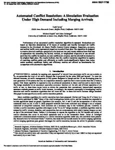
Post-simulation analysis of the conflicts delegated to TSAFE found that all of the delegated conflicts would have been solved without violating the separation standards. This result is summarized in row e of Table 5. However, because a conflict avoidance algorithm is not implemented in the ACES simulation environment, we do not have simulation data to support this analysis. We intend to validate this result once a conflict avoidance algorithm is incorporated into ACES. In many cases, especially at the higher traffic densities, the resolution algorithm was presented with conflicts with less than 2 min to first loss of separation (tlos) (see Figure 10). In a deterministic simulation environment such as the one used for this study, the majority of conflicts should have been detected at or near the 8-min range of the conflict detection algorithm, such as shown in the “1x” panel of Figure 10, where 23% of conflicts were detected 78 min prior to loss of separation, and another 30% were detected 6-7 min prior to loss of separation. Contrast these data with the 3x case, where 25% of conflicts were detected 1-2 min prior to first loss of separation. The frequency of “late” conflict detections presented an additional challenge to the 6 These cases of “late” conflict alerts are discussed in more detail later in this section.

35%

1x

2x

3x

30%

% of total detected conflicts

In cases where the algorithm failed to compute an acceptable resolution trajectory, the conflict was delegated to the conflict avoidance algorithm. As mentioned previously, conflict avoidance algorithms deliver expediency over efficiency. Specifically, they differ from conflict resolution algorithms by their expanded maneuvering envelope (e.g., maximum allowable bank angle, climb rate, etc.) and by their simpler, fail-safe architectures. In the Automated Airspace Concept (to which the conflict resolution algorithm being benchmarked belongs), the conflict avoidance function is called the Tactical Separation Assisted Flight Environment, or TSAFE. As shown in row d of Table 5, some conflicts had to be delegated to TSAFE. It is important to note that all of these delegated conflicts were first detected with less than two minutes until the first loss of separation.6 While it is possible for the conflict resolution algorithm to resolve a conflict in that short timeframe, the tighter maneuvering constraints imposed on the conflict resolution algorithm (as opposed to the conflict avoidance algorithm) make it difficult. Ultimately, system architects must decide the criteria for when to invoke conflict avoidance rather than relying on conflict resolution. These results may help inform that decision.

25% 20%

15% 10% 5% 0%