ADVANCED ELECTROMAGNETICS, VOL. 6, NO. 3, OCTOBER 2017
Fast Wideband Solutions Obtained Using Model Based Parameter Estimation with Method of Moments Fatih Kaburcuk Electrical and Electronics Engineering Department, Erzurum Technical University, Erzurum, Turkey E-mail:
[email protected],
[email protected]
Abstract Integration of the Model Based Parameter Estimation (MBPE) technique into Method of Moments (MOM) provides fast solutions over a wide frequency band to solve radiation and scattering problems. The MBPE technique uses the Padé rational function to approximate solutions over a wide frequency band from a solution at a fixed frequency. In this paper, the MBPE technique with MOM is applied to a thin-wire antenna. The solutions obtained by repeated simulations of MOM agree very well with the solutions obtained by MBPE technique in a single simulation. Therefore, MBPE technique according to MOM provides a remarkable saving in the computation time. Computed results show that solutions at a wider frequency band of interest are achieved in a single simulation.
1. Introduction A Model Based Parameter Estimation (MBPE) technique integrated into Method of Moments (MOM) is performed to obtain solutions at a wide frequency band from a solution at a fixed center frequency (𝑓 ) [1-7]. The technique integrated into MOM has also been studied to analyze two-dimensional scattering problems [8-10]. In this paper, a thin-wire antenna is analyzed using MBPE technique integrated into MOM to obtain solutions at any frequency of interest using the current distribution and its frequency derivatives at 𝑓 . The MBPE technique uses the current distribution and its frequency derivative at 𝑓 to obtain the model coefficients of the rational function. These model coefficients are used to obtain the current distribution at frequencies of interest away from 𝑓 . Using the current distribution at 𝑓 , the current distribution and input impedance of the thin wire antenna at any frequency of interest can be efficiently calculated. The computation time of the MOM is more than that of MBPE technique because the MOM simulation is performed for each frequency of interest. The normalized error of the solutions obtained using the MBPE technique respect to MOM is calculated to show the accuracy of the MBPE technique.
2. Procedure of Model Based Parameter Estimation with Method of Moments 2.1. Model Based Parameter Estimation Technique In the MBPE technique, 𝑖 current distribution ( 𝐼 ) is expressed by a rational function of frequency. The rational function is expressed as the ratio of two polynomials as follows: j Ni f j 0Nij f N N i1 f N i 2 f 2 Nin f n . (1) d i0 Di f Dij f j Di 0 Di1 f Di 2 f 2 Did f d n
Ii f
j 0
where 𝑓 is the frequency of interest, 𝑁 and 𝐷 are the model coefficients of numerator and denominator of the rational function, respectively. The high-order polynomials in both numerator and denominator of the rational function are used to obtain more accurate solutions over a wider frequency band. As an example, the current distribution having two expansion coefficients are expressed by rational functions of frequency as follows: n N fj N1 f j0 1 j N10 N11 f N12 f 2 N1n f n . (2) j d I f D1 f j0D1 j f 1 D11 f D12 f 2 D1d f d I f 1 2 n n I2 f N2 f j0N2 j f j N20 N21 f N22 f N2n f 2 d D2 f d D f j 1 D21 f D22 f D2d f 2 j j0
2.2. Calculation of Model Coefficients in the Rational Function The model coefficients 𝑁 ’s and 𝐷 ’s in (1) are obtained using both frequency and frequency derivative samples. Starting with (1) and differentiating 𝑘 times with respect to 𝑓 gives: I i f Di f N i f
I i' f Di f I i f Di' f N i' f I i' ( f ) Di ( f ) 2 I i' ( f ) Di' ( f ) I i ( f ) Di'' ( f ) N i'' ( f )
, (3)
k m k m I i k f Di f k I i k 1 f Di' f f I i f Di k m k I i' f Di k 1 f I i f Di k f N i k f
where
𝑘 𝑘−𝑚
is the binomial coefficient and the
superscripts represent the order of frequency derivative.
There are 𝑘 + 1 equations that are used to obtain the unknown model coefficients in (3). When the frequency derivatives of the current distribution are obtained at only center frequency (𝑓 ), Equation (3) can be written by substituting 𝑓 by 𝑓 − 𝑓 , where 𝑓 − 𝑓 shows the frequency shifting from 𝑓 . The following linear equations can be written after setting 𝑘 = 𝑛 + 𝑑 and 𝐷 = 1.
F k k F I i k Yij V j k Z jtm I t k m , m j 1 m 1 t 1
𝑘 is the binomial coefficient and the superscript 𝑚 represents the number of frequency derivative. It is realized from Eq. (11) that the derivatives and inverse of the moment matrix are required, each iterative derivative involves only the inverse moment matrix, and its derivative is not required. The model unknown coefficients 𝑁 ’s and 𝐷 ’s in (1) can be determined after replacing the current distribution 𝐼 and its 𝑘 derivatives at f0 given in (11) into (6). Substituting the variable 𝑓 by f−f0 in (1), 𝐼 can be written as: where
Ni 0 Ii0 N i1 I i 0 Di1 I i1 N i 2 I i1 Di1 I i 0 Di 2 I i 2
N in I i n 1 Di1 I i n 2 Di 2 I i n d Did I in
,
Ii f f 0
(4)
I in Di1 I i n 1 Di 2 I i n d 1 Did I i n1
where 1 P (5) Ii 0 P 0,1, , k , P! where 𝐼 is a function of frequency (𝑓 − 𝑓 ). Finally, the following matrix equation is obtained from the linear equations in (4) to determine the unknown model coefficients in (1). I iP
0 0 0 ⋮
⋯ ⋯ ⋱ ⋯
1 0 ⋮ 0
0 −𝐼 −𝐼 ⋮ −𝐼 ( −𝐼 ⋮ −𝐼 (
)
)
0 0 −𝐼 ⋮ −𝐼 ( −𝐼 ( ⋮ −𝐼 (
⋯ ⋯ ⋯ ⋱ ⋯ ⋯ ⋱ ⋯
) )
)
0 0 0 ⋮
𝑁 ⎤⎡ ⎥ ⎢𝑁 ⎥ ⎢𝑁 ⋮ −𝐼 ( ) ⎥ ⎢𝑁 ⎥⎢ −𝐼 ( )⎥ ⎢𝐷 ⋮ ⎥⎢ ⋮ −𝐼 ( ) ⎦ ⎣𝐷
𝐼 ⎤ ⎡ 𝐼 ⎥ ⎢ 𝐼 ⎥ ⎢ ⎥=⎢ ⋮ ⎥ ⎢ 𝐼 ⎥ ⎢𝐼 ( ⎥ ⎢ ⋮ ⎦ ⎣ 𝐼
2
⎤ ⎥ ⎥ ⎥. ⎥ )⎥ ⎥ ⎦
Z ij
j 30 e jkR1 e jkR2 e jkr 2cos kd sin kd R1 R2 r
𝑟 = √𝑎 + ℎ , 𝑅 = 𝑎 + (ℎ − 𝑑) , and 𝑅 = 𝑎 + (ℎ + 𝑑) , where 𝑅 , 𝑅 , and 𝑟 are defined for each segment of the thin wire antenna as illustrated in Fig. 1, d is the length of a segment of the wire, a is the radius of the thin wire, and 𝑘 is the wave number.
(6)
𝑧
The well-known MOM equation
Z I ij
j
Vi ,
j 1
for 1, 2,, k ,
𝑎
(7) 𝑑
where F is the order of the frequency dependent moment matrix Z, and 𝑉 and 𝐼 are the source and current distribution vector, respectively. 𝑖 current distribution (𝐼 ) in MOM can be calculated using the inverse moment matrix (Y) as follows: F
I i YijV j ,
𝑑
j 1
ij
I 'j Z ij' I j V j' .
ℎ
𝑅
Figure 1: Geometry of a segment of a thin wire antenna for the Moment matrix calculation.
(8)
j 1
F
𝑅 𝑟
𝑦
First derivative of (7) with respect to frequency, it can be obtained
Z
, (13)
where
2.3. Integration MBPE into MOM F
n
The Moment matrix used in the calculation of the current distribution over a thin wire antenna are expressed here. The antenna is divided into 81 segments. The piecewise sinusoids are chosen as expansion functions and point matching is used for testing function. The moment matrix are calculated analytically given in [11]. The Moment matrix is expressed as follows:
I i k 1 Di1 I i k 2 Di 2 I i k d Did I ik
⋯ ⋯ ⋯ ⋱
Ni 0 Ni1 f f0 Ni 2 f f0 Nin f f0 .(12) 2 d 1 Di1 f f0 Di 2 f f0 Did f f0
2.4. Expression of the Moment Matrix (Z)
1 0 ⋯ ⎡ 0 1 ⋯ ⎢0 0 1 ⎢⋮ ⋯ ⋯ ⎢ ⎢0 0 ⋯ ⎢0 0 ⋯ ⎢⋮ ⋯ ⋯ ⎣0 0 ⋯
(11)
3. Numerical Results A thin-wire antenna of length L and radius 𝑎=L/148.4 which is fed by a delta-gap source is analyzed using the MBPE with MOM. The current distribution and input impedance of the thin-wire antenna at any frequency of interest away from f0 are calculated. The solutions calculated by MOM using a point-by-point approach are compared with the results obtained by MBPE technique with both frequency and different order frequency derivative samples at f0=300 MHz. All of the simulations presented in this paper are performed using MATLAB. To prove the convergence of the solutions
(9)
Then the first derivative of the 𝑖 current distribution is expressed by F F (10) I i' Yij V j' Z 'jt I t . j 1 t 1 In general, the 𝑘 frequency derivative of the 𝑖 current distribution is given by
14
obtained using MBPE technique and MOM with a point-bypoint approach, a normalized error is defined as: MBPE MOM Normalized error maximum MOM
2
.(14) 100%
1.5 Error(%)
In all simulation, the current distributions are calculated at limit frequencies where the normalized error is less than 2%. Fig. 2 show the current distributions on the antenna computed using MOM and MBPE technique by taking 9 derivatives (n = 5, d = 4) at f = 0.02f0 and f = 2.4f0, respectively, when the length of the thin wire antenna is taken to be 0.5m. The numerical comparison shows that result obtained using MOM is in a good agreement with that obtained using MBPE technique. It can be seen from Fig. 2 that MBPE technique with MOM provides accurate results using the solution obtained by MOM at f0. Good agreements between the current distributions obtained using MBPE and MOM at all frequencies between 0.02f0 and 2.4f0 are achieved. The normalized error over the frequency band is shown Fig. 3. It can be realized that the error is increasing when the frequency is moving away from the center frequency.
1
0.5
0
0
0.4
0.8 1.2 1.6 Antenna Length / Wavelength
2
2.4
Figure 3: The normalized error for the current distributions. To show the performance of the MBPE technique and MOM, the computation time of MBPE technique and MOM versus number of frequencies is shown in Fig. 4. The computation time of MBPE technique is not significantly increasing when the number of frequencies in the simulation is increased whereas that of MOM is increasing significantly because the MOM simulation is performed for each frequency of interest.
0.1
(a) 0.08
Simulation Time (second)
Miliampere (mA)
30 0.06
0.04 M oM
0.02
0
th
M BPE (9 FD)
0
0.1
0.2 0.3 Antenna Length (m)
0.4
0.5
25 20 15 MOM MBPE
10 5
6
(b)
0
M oM
5
th
Miliampere (mA)
M BPE (9 FD)
20
40
60
80 100 120 140 160 180 200 220 Number of Frequencies
Figure 4: The consumed computation time of MBPE technique and MOM simulation when increasing the number of frequencies.
4 3
Fig. 5 show the current distributions on the antenna at f =0.4f0 and f =1.6f0 when the length of the thin-wire antenna L is 1m. The comparison between the solid curves computed using MOM and the dashed curves computed using MBPE technique shows that good agreement is achieved. It can be seen from Fig. 5 that MBPE technique taking 9 derivatives (n = 5, d = 4) provides accurate results using the solution obtained by MOM at f0. The normalized maximum error over the frequency band is shown Fig. 6.
2 1 0
0
0
0.1
0.2 0.3 Antenna Length (m)
0.4
0.5
Figure 2: Current distribution on the thin wire antenna at a) f =0.02 f0 and b) f =2.4 f0.
15
10
800
Antenna Input Impedance (ohm)
(a)
Miliampere (mA)
8
6 MoM
4
MBPE (9th FD) 2
0
0.2
0.4 0.6 Antenna Length (m)
0.8
1
(b) 4 Miliampere (mA)
MBPE (5th FD) MBPE (9th FD)
400 200 0 -200 -400
0
0.25
0.5
0.75 1 1.25 1.5 1.75 Antenna Length / Wavelength
2
2.25
2.5
Figure 7: Input impedance of the thin-wire antenna calculated regular MOM and MBPE technique with 3th, 5th and 9th frequency derivative.
5
4. Conclusions Integration of the MBPE technique into MOM can provide solutions over a wide frequency band. In this paper, a thinwire antenna is analyzed to obtain solutions over a wide frequency band. The current distribution and input impedance of the antenna at frequencies of interest away from the center frequency f0 obtained using MOM are in very good agreement with that obtained using MBPE technique. The computation time consumed by MOM is more than that consumed by MBPE technique when the number of frequencies is increased in the simulation. It was realized that more frequency derivatives provide more accurate results over a wide frequency band.
3
2
1
MoM MBPE (9th FD)
0
MBPE (3th FD)
600
-600
0
MoM
0
0.2
0.4 0.6 Antenna Length (m)
0.8
1
Figure 5: Current distribution on the thin wire antenna at a) f =0.4fo and b) f =1.6fo.
References
1.8
[1] G. J. Burke, E. K. Miller, S. Chakrabarti, and K. Demarest, “Using Model-Based Parameter Estimation to Increase the Efficiency of Computing Electromagnetic Transfer functions,” IEEE Transaction on Magnetics, Vol. 25, No. 4, pp. 2807–2809, July 1989. [2] S. Chakrabarti, R. Ravichander, E. K. Miller, J. R. Auton, and G. J. Burke, “Applications of Model-Based Parameter Estimation in Electromagnetic Computations”, Circuit and Systems, Proceeding of the 32nd Midwest Symp. on, Vol. 2, pp. 712–715, 1990. [3] E. K. Miller, “Using Model-Based Parameter Estimation for Characterising Broadband Electromagnetic Transfer Functions”, Asia-Pasific Microwave Conference, Vol. 1, pp. 451–454, Aug. 1992. [4] E. K. Miller, “Model-Based Parameter Estimation in Electromagnetics: I-Background and Theoretical Development”, IEEE Antennas and Propagation Magazine, Vol. 40, No. 1, pp. 42–52, Feb. 1998. [5] E. K. Miller, “Model-Based Parameter Estimation in Electromagnetics: II-Application to EM Observables”, IEEE Antennas and Propagation Magazine, Vol. 40, No.2, pp. 51–65, April 1998.
1.5
E rro r (% )
1.2 0.9 0.6 0.3 0 0.4
0.6
0.8 1 1.2 Antenna Length / Wavelength
1.4
1.6
Figure 6: The normalized error for the current distributions. Fig. 7 shows the input impedance of the thin-wire antenna obtained by MOM and MBPE technique with 3, 5, and 9 derivatives. It can be seen from Fig. 7 that more accurate results are achieved when increasing the number of derivatives. The computation time of MBPE technique is 0.67 s whereas that of the conventional MOM is 32.55 s because the MOM simulation is performed for each frequency of interest. Therefore, the MBPE technique provides remarkable reduction in the computation time and solutions at any frequency of interest in a single simulation.
16
[6] E. K. Miller, “Model-Based Parameter Estimation in Electromagnetics: III-Application to EM Integral Equations”, IEEE Antennas and Propagation Magazine, Vol. 40, No.3, pp. 49–66, June 1998. [7] R. J. Reddy, “Application of Model Based Parameter Estimation for RCS Frequency Response Calculations Using Method of Moments”, NASA, 1998. [8] X. Yang and E. Arvas, “Use of frequency-derivative information in two- dimensional electromagnetic scattering problems,” Proc. Inst. Elect. Eng., pt. H, vol. 138, no. 4, pp. 269–272, Aug. 1991. [9] H. Son, J.R.Mautz, and E. Arvas, “Use of Model-Based Parameter Estimation for Fast RCS Computation of a Conducting body of Revolution over a Frequency Band,” Applied Computational Electromagnetics Society Journal, pp. 65–72, March 2004. [10] F. Kaburcuk, S. Arvas, E. Arvas, and J. K. Lee, “Wideband information in MOM obtained from narrowband data,” Ultra-Wideband (ICUWB), 2012 IEEE International Conference on. IEEE, 2012. [11] E.C. Jordan and K. G. Balmain, Electromagnetic Waves and Radiating Systems, 2nd ed. Englewood Cliffs, NJ: Prentice-Hall Inc., 1968, pp. 333.
17