Locally Compressed Suffix Arrays - CiteSeerX

Locally Compressed Suffix Arrays Rodrigo González and Gonzalo Navarro Dept. of Computer Science, University of Chile. {rgonzale,gnavarro}@dcc.uchile.cl

Compressed text (self-)indexes have matured up to a point where they can replace a text by a data structure that requires less space and, in addition to giving access to arbitrary text passages, support indexed text searches. At this point those indexes are competitive with traditional text indexes (which are very large) for counting the number of occurrences of a pattern in the text. Yet, they are still hundreds to thousands of times slower when it comes to locating those occurrences in the text. In this paper we introduce a new, local, compression scheme for suffix arrays which permits locating the occurrences extremely fast, while still being much smaller than classical indexes. The core of our contribution is the identification of the regularities exploited by the compression based on function Ψ, used for long time in compressed text indexing, with those exploited by Re-Pair on the differential suffix array. The latter enjoys the locality properties that the former methods lack. As another consequence of this locality, we show that our index can be implemented in secondary memory, where its access time improve thanks to compression, instead of worsening as is the norm in other self-indexes. Finally, some byproducts of our work, such as a compressed dictionary representation for Re-Pair, can be of independent interest. Categories and Subject Descriptors: F.2.2 [Analysis of algorithms and problem complexity]: Nonnumerical algorithms and problems—Pattern matching, Computations on discrete structures, Sorting and searching; H.2.1 [Database management]: Physical design—Access methods; H.3.2 [Information storage and retrieval]: Information storage—File organization; H.3.3 [Information storage and retrieval]: Information search and retrieval—Search process General Terms: Algorithms Additional Key Words and Phrases: Compressed text indexing, compressed suffix arrays, Re-Pair

1. INTRODUCTION AND RELATED WORK Compressed text indexing has become a popular alternative to cope with the problem of giving indexed access to large text collections without using up too much space. Reducing space is important because it gives one the chance of maintaining the whole collection in main memory. The current trend in compressed indexing is full-text compressed self-indexes [Navarro and M¨ akinen 2007; Ferragina and Manzini 2005; Grossi et al. 2003; Sadakane 2003; Navarro 2004; Ferragina et al. 2007]. Such a self-index (for short) replaces the text by providing fast access to arbitrary text substrings, and in addition gives indexed access to the text by supPartially supported by Yahoo! Research grant “Compressed data structures” (Chile) and Millennium Nucleus Center for Web Research, Grant P04-067-F, Mideplan, Chile. An early partial version of this article appeared in Proc. 18th Combinatorial Pattern Matching (CPM), LNCS 4580, pp. 216–227, 2007. Permission to make digital/hard copy of all or part of this material without fee for personal or classroom use provided that the copies are not made or distributed for profit or commercial advantage, the ACM copyright/server notice, the title of the publication, and its date appear, and notice is given that copying is by permission of the ACM, Inc. To copy otherwise, to republish, to post on servers, or to redistribute to lists requires prior specific permission and/or a fee. c 20YY ACM 0000-0000/20YY/0000-0001 $5.00

ACM Journal Name, Vol. V, No. N, Month 20YY, Pages 1–27.

2

·

porting fast search for the occurrences of arbitrary patterns. These indexes take little space, usually from 30% to 150% of the text size (note that this includes the text). This is to be compared with classical indexes such as suffix trees [Weiner 1973] and suffix arrays [Manber and Myers 1993], which require at the very least 10 and 4 times, respectively, the space of the text, plus the text itself. In theoretical terms, to index a text T = t1 . . . tn over an alphabet of size σ, the best self-indexes require nHk + o(n log σ) bits for any k ≤ α logσ n and any constant 0 < α < 1, where Hk ≤ log σ is the k-th order empirical entropy of T [Manzini 2001; Navarro and M¨ akinen 2007]1. Just the uncompressed text alone would need n log σ bits, and classical indexes require O(n log n) bits on top of it. The search functionality is given via two operations. The first is, given a pattern P = p1 . . . pm , count the number of times P occurs in T . The second is to locate the occurrences, that is, list their positions in T . Current self-indexes achieve a counting performance that is comparable in practice with that of classical indexes. In theoretical terms, for the best self-indexes the complexity is O(m(1 + logloglogσ n )) and even O(1 + logm n ), compared to O(m log σ) of suffix trees and O(m log n) or σ O(m+log n) of suffix arrays. Locating, on the other hand, is far behind, hundreds to thousands of times slower than their classical counterparts. While classical indexes pay O(occ) time to locate the occ occurrences, self-indexes pay O(occ log ε n), where ε can in theory be any constant larger than zero but is in practice larger than 1. Worse than that, the memory access patterns of self-indexes are highly nonlocal, which makes their potential secondary-memory versions rather unpromising. Extraction of arbitrary text portions is also quite slow and non-local compared to having the text directly available as in classical indexes. The only implemented self-index which has more local accesses and faster locate is the LZ-index [Navarro 2004], yet its counting time is not competitive. In this paper we propose a suffix array compression technique that builds on wellknown regularity properties that show up in suffix arrays when the text they index is compressible (more precisely, the runs in the Ψ function of the suffix array, or which is the same, the number of equal-letter runs in the Burrows-Wheeler transform of the text [Navarro and M¨ akinen 2007]). This regularity has been exploited in several ways in the past [Mäkinen 2003; Grossi and Vitter 2006; Grossi et al. 2003; Sadakane 2003; M¨ akinen and Navarro 2005], but we present a completely novel technique to take advantage of it. We represent the suffix array using differential encoding, which converts the regularities into true repetitions. Those repetitions are then factored out using Re-Pair [Larsson and Moffat 2000], a compression technique that builds a dictionary of phrases and permits fast local decompression using only the dictionary (whose size one can limit at will, at the expense of losing some compression). We then introduce novel techniques to further compress the Re-Pair dictionary, which can be of independent interest. We also use specific suffix array properties to obtain a much faster compression method that loses just up to 1% of compression ratio. Our so-called locally compressed suffix array (LCSA) is shown to reduce the suffix array to 20–70% of its original size, depending on the compressibility of various text types. This reduced index can still extract any portion of the suffix array very fast 1 In

this paper log stands for log2 .

ACM Journal Name, Vol. V, No. N, Month 20YY.

·

3

by adding a small set of sampled absolute values. By using the deep connection with function Ψ, we prove that the size of the result is O(Hk log H1k n log n) + o(n) bits2 for any k ≤ α logσ n and any constant 0 < α < 1. Note that this reduced suffix array is not yet a self-index as it cannot reproduce the text. This structure can be used in two ways. One way is to attach it to a self-index able of counting, which in this process identifies as well the segment of the (virtual) suffix array where the occurrences lie. We can then locate the occurrences by decompressing that segment using our structure. The result is a self-index that needs 1–3 times the text size (that is, considerably larger than current self-indexes but also much smaller than classical indexes) and whose counting and locating times are competitive with those of classical indexes, far better for locating than current self-indexes. In theoretical terms, assuming for example the use of an alphabet-friendly FM-index [Ferragina et al. 2007] for counting, our index needs O(Hk log H1k n log n+ n) bits of space, counts in time O(m(1 + logloglogσ n )) and locates the occ occurrences of P in time O(occ + log n). In practice, even letting classical self-indexes use the same amount of space to speed up their locating time, they are much slower than our LCSA for reporting more than a few occurrences (2–10). A second and simpler way to use the structure is, together with the plain text, as a replacement of the classical suffix array. In this case we must not only use it for locating the occurrences but also for binary searching. The binary search is done over the samples first and then we decompress the area between two consecutive samples to finish the search. This yields a very practical alternative requiring 0.8– 2.4 times the text size (as opposed to 4) plus the text, in exchange for being just 2–28 times slower for locating. On the other hand, if the text is very large, even a compressed index must reside on disk. Performing well on secondary memory with a compressed index has proved extremely difficult, because of their non-local access pattern. Thanks to its local decompression properties, our reduced suffix array performs very well on secondary memory. It needs the optimal ⌈ occ B ⌉ disk accesses for locating the occ occurrences, being B the disk block size measured in integers. On average, if the compression ratio (compressed divided by uncompressed suffix array size) is 0 ≤ c ≤ 1, we perform ⌈ c·occ B ⌉ accesses. That is, our index actually performs better, not worse (as it seems to be the norm), thanks to compression. We show how to build this structure almost I/O-optimally in secondary memory for large suffix arrays. Achieving compressed indexes able of counting in competitive time was the first important breakthrough in this area. We believe our work is a first important step towards compressed indexes with practical locating times. This is up to date the major concern for adopting compressed indexes in practical applications. This paper is organized as follows. In Section 2 we describe our LCSA. In section 3 we analyze its compression ratio, relating it to the compressibility of the text. In Section 4 we show how to use the LCSA as part of various indexing schemes. In Section 5 we carry out several experimental tunings and comparisons with alternative compressed and classical indexes. In Section 6 we give a secondary memory n result is meaningful for Hk = o(1). The general result is O(N (1 + log N ) log n) bits, where N is the number of runs in Ψ. Acording to M¨ akinen and Navarro [2005], N ≤ min(n, nHk + σk ) for any k.

2 This


4

·

construction algorithm for the LCSA when the structures do not fit in main memory. Finally, in Section 7 we give our conclusions and future work directions. 2. A LOCALLY COMPRESSED SUFFIX ARRAY (LCSA) Given a text T = t1 . . . tn over alphabet Σ of size σ, where for technical reasons we assume tn = $ is smaller than any other character in Σ and appears nowhere else in T , a suffix array A[1, n] is a permutation of [1, n] such that TA[i],n ≺ TA[i+1],n for all 1 ≤ i < n, being “≺” the lexicographical order. By Tj,n we denote the suffix of T that starts at position j. Since all the occurrences of a pattern P = p1 . . . pm in T are prefixes of some suffix, a couple of binary searches in A suffice to identify the segment in A of all the suffixes that start with P , that is, the segment pointing to all the occurrences of P . Thus the suffix array permits counting the occurrences of P in O(m log n) time and reporting the occ occurrences in O(occ) time. With an additional array of integers, the counting time can be reduced to O(m + log n) [Manber and Myers 1993]. Suffix arrays turn out to be compressible whenever T is. The k-th order empirical entropy of T , Hk [Manzini 2001], shows up in A in the form of large segments A[i, i + ℓ] that appear elsewhere in A[j, j + ℓ] with all the values shifted by one position, A[j + s] = A[i + s] + 1 for 0 ≤ s ≤ ℓ. Actually, one can partition A into runs of maximal segments that appear repeated (shifted by 1) elsewhere, and the number of such runs is at most nHk + σ k for any k [Mäkinen and Navarro 2005; Navarro and M¨ akinen 2007]. This property has been used several times in the past to compress A. M¨ akinen’s Compact Suffix Array (CSA) [Mäkinen 2003] replaces runs with pointers to their definition (copy) elsewhere in A, so that the run can be recovered by (recursively) expanding the definition and shifting the values. M¨ akinen and Navarro [2005] use the connection with FM-indexes (runs in A are related to equal-letter runs in the Burrows-Wheeler transform of T , basic building block of FM-indexes) and runlength compression. Yet, the most successful technique to take advantage of those regularities has been the definition of function Ψ(i) = A−1 [A[i] + 1] (or A−1 [1] if A[i] = n). It can be seen that Ψ(i) = Ψ(i − 1) + 1 within runs of A, and therefore a differential encoding of Ψ is highly compressible [Grossi et al. 2003; Sadakane 2003]. 2.1 Basic LCSA Idea We present a completely different method to compress A. We first represent A in differential form A′ : Definition 1. Let A[1, n] be an array of integers. Then we define A′ [1, n] as follows: A′ [1] = A[1] and A′ [i] = A[i] − A[i − 1] for all 1 < i ≤ n. The next simple lemma shows that runs of A become true repetitions in A′ . Lemma 1. Consider a run of A of the form A[j + s] = A[i + s] + 1 for 0 ≤ s ≤ ℓ. Then A′ [j + s] = A′ [i + s] for 1 ≤ s ≤ ℓ. Proof. A′ [j + s] = A[j + s] − A[j + s − 1] = (A[i + s] + 1) − (A[i + s − 1] + 1) = A[i + s] − A[i + s − 1] = A′ [i + s]. ACM Journal Name, Vol. V, No. N, Month 20YY.

·

5

We can now exploit those repetitions using any classical compression method. In particular, we seek a method that allows fast local decompression of A′ . We resort to Re-Pair [Larsson and Moffat 2000], a dictionary-based compression method based on the following algorithm: (1) Identify the most frequent pair A′ [i]A′ [i + 1] in A′ , let ab be such pair. (2) Create a new integer symbol s, larger than all existing symbols in A′ , and add rule s → ab to a dictionary R. (3) Replace every occurrence of ab in A by s.3 (4) Iterate until every pair has frequency 1. The result of the compression algorithm is the dictionary of rules R plus the sequence C of (original and new) symbols into which A′ has been compressed. Note that R can be easily stored as a vector of pairs, so that rule s → ab is represented by R[s − n] = a : b. Any portion of C can be easily decompressed in optimal time and fast in practice. To decompress C[i], we first check if C[i] ≤ n. If it is, then it is an original symbol of A′ and we are done. Otherwise, we obtain both symbols from R[C[i] − n], and expand them recursively (they can in turn be original or created symbols, and so on). We reproduce u cells of A′ in O(u) time, and the accesses pattern is local if R is small. Since R grows by 2 integers (a, b) for every new pair, we could stop creating pairs when the most frequent one appears only twice. R can be further reduced by preempting this process, which trades its size for overall compression ratio. Apart from R and C, we need a few more structures to recover the values of A: —An array S such that S[i] = A[i· l], that is, a sampling of absolute values of A at regular intervals l. —A bitmap L[1, n], marking the positions where each symbol of C (which could represent several symbols of A′ ) starts in A′ . —o(n) further bits to answer rank queries on L in constant time [Jacobson 1989; Navarro and M¨ akinen 2007], where rank(L, i) is the number of 1’s in L[1, i]. With this structure, the algorithm to retrieve A[i, j] is as follows: (1) Check if there is a multiple of l in [i, j], extending i to the left or j to the right to include such a multiple if necessary. (2) Use the mechanism to decompress one symbol in C (described above) to obtain A′ [i, j], by expanding C[rank(L, i), rank(L, j)]. We expand from right to left, so the first symbol may be not totally expanded. (3) Use any absolute sample of A included in S[⌊i/l⌋, ⌊j/l⌋] to obtain, using the differences in A′ [i, j], the values A[i, j]. (4) Return the values in the original requested interval [i, j]. 3 If a = b it might be impossible to replace all occurrences, e.g. aa in aaa. But, in such case, one can at least replace each other occurrence in a row.


6

·

The overall time complexity of this decompression is the output size plus what we have expanded the interval to include a multiple of l (i.e., O(l)) and to ensure an integral number of symbols in C. The latter can be controlled by limiting the length of the uncompressed version of the symbols we create. 2.2 Compression using Ψ A weak point of using Re-Pair is its compression speed and space usage. Re-Pair can be implemented in O(n) time, but this needs too much space [Larsson and Moffat 2000]. Instead of using the original Re-Pair, we opt for a technique that needs less space and usually runs in O(n log n) time. This technique is not too interesting (and we do not describe it) except as a control value to test our more important contribution: We introduce a fast approximate technique specialized to compressing suffix arrays A. We show that Ψ (which is easily built in O(n) time from A) can be used to obtain a much faster compression algorithm, which in practice compresses almost as much as the original Re-Pair. Recall that Ψ(i) tells where in A is the value A[i]+1. The idea is that, if A[i, i+ℓ] is a run such that A[j + s] = A[i + s] + 1 for 0 ≤ s ≤ ℓ (and thus A′ [j + s] = A′ [i + s] for 1 ≤ s ≤ ℓ), then Ψ(i + s) = j + s for 0 ≤ s ≤ ℓ. Thus, by following permutation Ψ we have a good chance of finding repeated pairs in A′ . The basic idea is to choose the pairs while following permutation Ψ, cycling several times over A′ , until no further replacements can be done. This does not guarantee to choose the same pairs of the original Re-Pair, but we expect them to be sufficiently good. Data Structures. To compress using Ψ we need only two arrays and one bitmap. —An array D[1, n], which initially stores the suffix array of text T in differential form, D[i] = A′ [i] ∀i. At the end, we compact the valid values of D to obtain C. —An array P [1, n], which initially stores the values of function Ψ of text T , P [i] = Ψ(i) ∀i. —The bitmap L[1, n], where L[i] = 1 indicates that D[i] is a valid value. In the beginning L[i] = 1 ∀i. At the end, L can be preprocessed for rank queries and is ready for querying. When we replace a pair with a new symbol, array D becomes sparse. A way to find the next valid symbol in constant time is as follows: If a valid symbol D[i] is followed by an invalid symbol D[i + 1] (that is, L[i, i + 1] = 10), then D[i + 1] can be used to store the distance i′ − i to the next valid symbol D[i′ ] (we use i′ with this meaning, for any i, in the next algorithm description). This permits obtaining any pair of the sparse D in constant time. In practice, it turns out to be faster to calculate i′ = selectnext(L, i), which returns the position of the first 1 in L[i + 1, n], by scanning the bitmap word-wise. Algorithm. We make a number of passes over D. Each pass starts at i = 1 (where value A′ [1] = A[1] = n will not be replaced by Re-Pair as it is unique). For each i visited along the pass, we see if D[i]D[i′ ] = D[P [i]]D[P [i]′ ]. If this does not hold, we move on to i ← P [i] and iterate. If, instead, equality holds, we start a chain of replacements: We add a new pair s → D[i]D[i′ ] to R, make the replacements at i and P [i] (invalidating i + 1 and P [i] + 1), and move on to i ← P [i], continuing the ACM Journal Name, Vol. V, No. N, Month 20YY.

·

7

replacements until the pair changes. In this process, when a position P [j] becomes invalid, we set P [j] ← P [P [j]], so that the position is skipped in the next pass. When the pair finally changes, that is, D[i]D[i′ ] 6= D[P [i]]D[P [i]′ ], we restart the process with i ← P [i], looking again for a new pair to create. We keep running passes over D (using P ) as long as we replace at least αn′ pairs in a pass, where 0 < α < 1 is a constant and n′ is the number of valid elements in D in the previous pass. Figure 1 shows a more detailed pseudocode. Algorithm Compress(D, P , α) s ← n, R ← ∅ for i ← 1 . . . n do L[i] ← 1 n′ ← n, rep ← 0 do n′ ← n′ − rep rep ← 0 j ← 1, j ′ ← selectnext(L, j) do do i ← j, i′ ← j ′ while L[P [i]] = 0 do P [i] ← P [P [i]] j ← P [i], j ′ ← selectnext(L, j) while j 6= 1 and D[i]D[i′ ] 6= D[j]D[j ′] if j 6= 1 then ab ← D[i]D[i′ ], s ← s + 1, R ← R ∪ {s → ab} D[i] ← s, L[i′ ] ← 0, rep ← rep + 1 do D[j] ← s, L[j ′ ] ← 0, rep ← rep + 1 i ← j, i′ ← j ′ while L[P [i]] = 0 do P [i] ← P [P [i]] j ← P [i], j ′ ← selectnext(L, j) while j 6= 1 and ab = D[j]D[j ′] while j 6= 1 while (rep > αn′ ) j←1 for i ← 1 . . . n do if L[i] = 1 then D[j] ← D[i], j ← j + 1 return (C[1, n′ ] = D, R, L) Fig. 1.

Algorithm to compress D = A′ using P = Ψ in O(n) time.

Cost. Let ni be the number of elements in the i-th pass, then ni+1 ≤ (1 − α)ni . Since n0 = n, it holds ni ≤ (1 − α)i n. The i-th pass costs O(ni ) time. Let k be the number of passes doing more than αn′ replacements. So the total cost is at most k X X 1 (1 − α)i n + (1 − α)k n ≤ n (1 − α)i + (1 − α)k n ≤ 1+ n = O(n). α i=0 i≥0

Thus our algorithm achieves linear time while requiring only the space for D (overwritten on A′ and finally leaving there C), for P (overwritten on Ψ), and for L (which is also needed in the final structure). It is also simple and fast in practice. 2.3 Stronger Compression based on Ψ The only advantage of using the original Re-Pair is that it yields better compression and enforces the property that each new rule in the dictionary removes no more ACM Journal Name, Vol. V, No. N, Month 20YY.

8

·

pairs than the previous rule. The latter comes from the fact that the pairs in RePair are replaced in decreasing order of frequency. This prevents less frequent pairs to break longer chains of replacements. We now modify the algorithm that uses Ψ to obtain compression ratios as close to Re-Pair’s as desired, at the expense of O(n log n) complexity (multiplied by a constant that increases as the compression ratio improves). The key idea is to replace longer chains first. Algorithm. The algorithm is as follows: —We make one pass searching for the longest chain of equal pairs obtained by following Ψ, let f be its length. —We apply the previous algorithm, yet we only replace the chains of length at least t0 = δ · f , where 0 < δ < 1 is a constant. —Again we apply the previous algorithm using t1 = δ · t0 then t2 = δ · t1 and so on, until ti ≤ γ. At this point we decrement ti one by one until we reach ti = 1. Here γ is another parameter. Cost. We already know that the total cost of all passes that replace more than (1 − α)n′ elements adds up to O(n). The number of passes where we replace less than (1 − α)n′ pairs, on the other hand, is at most logδ f + γ. This is, logδ f for the part where t(·) decreases by a δ fraction, plus γ for the part where t(·) decreases one by one. Thus the total cost is at most: 1 n + (logδ f + γ) n. α Now, if we choose a constant s, α = 1/(s· log n), and γ = log n, the total time is O(n log n). Choosing other values of s, δ and γ we obtain better complexities, but worsen the compression quality. Within O(n log n) complexity, we can improve the compression ratio by tuning δ and s. 2.4 Compressing the Dictionary We now develop a technique to reduce the dictionary of rules R without affecting C. This can be of independent interest for Re-Pair in general. We note that the dictionary compression methods in the original Re-Pair article [Larsson and Moffat 2000] achieve much more compression. The advantage of our scheme is that we can decompress parts of the text without uncompressing the dictionary. This permits handling larger dictionaries in main memory. A first observation is that, if we have a rule s → ab and s is only mentioned in another rule s′ → sc, then we could perfectly remove rule s → ab and rewrite s′ → abc. This gives a net gain of one integer, but now we have rules of varying length. This is easy to manage, but we prefer to go further. We develop a technique that permits eliminating every rule definition that is used within R, once or more, and gain one integer for each such rule eliminated. The key idea is to write down explicitly the binary tree formed by expanding the definitions (by doing a preorder traversal and writing 1 for internal nodes and 0 for leaves), so that not only the largest symbol (tree root) can be referenced later, but also any subtree. For example, assume the rules R = {s → ab, t → sc, u → ts}, and C = tub. We could first represent the rules by the bitmap RB = 100100100 (where s corresponds ACM Journal Name, Vol. V, No. N, Month 20YY.

·

9

to position 1, t to 4, and u to 7) and the sequence RS = ab1c41 (we are using letters for the original symbols of A′ , and bitmap positions as the identifiers of created symbols). We express C as 47b. To expand, say, 4, we go to position 4 in RB and compute rank0 (RB , 4) = 2 (number of zeros up to position 4, rank0 (i) = i − rank(i)). Thus the corresponding symbols in RS start at position 2 + 1 = 3. We extract one new symbol from RS for each new zero we traverse in RB , and stop when the number of zeros traversed exceeds the number of ones (this means we have completed the subtree traversal). This way we obtain the definition 1c for symbol 4. More generally, R can be seen as R = {s1 → a1 b1 , s2 → a2 b2 , . . . , sk → ak bk }, where indeed sk = n + k (as n = A′ [1] = A[1] is the maximum value in A′ ). Thus, we write down RB , RS and the new C as follows (note that positions in RB are written in RS shifted by n to distinguish them from the original symbols): —RB = (100)k . —RS = a1 b1 a2 b2 . . . ak bk = r1 r2 r3 . . . r2k , except that if ri > n we set it to ri = n + 1 + 3(ri − n − 1), so that they point to the 1’s in RB . —C = c1 c2 . . . cn′ undergoes the same transformation: if ci > n, we set it to ci = n + 1 + 3(ci − n − 1). Let us now reduce the dictionary, in our example, by expanding the definition of s within t (even if s is used elsewhere). The new bitmap is RB = 11000100 (where t = 1, s = 2, and u = 6), the sequence is RS = abc12, and C = 16b. We can now remove the definition of t by expanding it within u. This produces the new bitmap RB = 1110000 (where u = 1, t = 2, s = 3), the sequence RS = abc3 and C = 21b. Further reduction is not possible because u’s definition is only used from C.4 At the cost of storing at most 2|R| bits (for RB ), we can reduce R by one integer for each definition that is used at least once within R. The reduction can be easily implemented in linear time, avoiding the successive renamings of our example, as follows: We first check for each rule if it is used within R, marking this in a bitmap U . Then we traverse R and only write down (the bits of RB and the sequence RS for) the entries that are not used within R. We recursively expand those entries, appending the resulting tree structure to RB and leaf identifiers to RS . Whenever we find a created symbol that does not yet have an identifier, we give it as identifier the current position in RB and recursively expand it. We store these new identifiers in an array N V . Otherwise the expansion finishes and we write down a leaf (a "0") in RB and the identifier in RS . Then we rewrite C using the renamed identifiers. Figure 2 shows detailed pseudocode. We can further compress the dictionary, if we take into account that a rule only uses previous rules or original symbols. That is, the i-th rule can only point to elements with representation of length ⌈log2 i⌉ bits. With a simple arithmetic computation we can directly access any rule. Another way to further compress the dictionary, yet with a time penalty, is as follows: Instead of using the position i of a rule inside bitmap RB , use j = 4 It is tempting to replace u in C, as it appears only once, but our example is artificial: A symbol that is not mentioned in R must appear at least twice in C.


10

·

Algorithm Compress Dictionary(R = {s1 → a1 b1 , . . . , sk → ak bk }, C = c1 . . . cn′ ) for i ← 1 . . . k do U [i] ← 0 for i ← 1 . . . k do if ai > n then U [ai − n] ← 1 if bi > n then U [bi − n] ← 1 for i ← 1 . . . k do N V [i] ← 0 j ← 1, RB ← hi, RS ← hi LRB ← 0 // length in bits of bitmap RB for j ← 1 . . . k do if U [j] = 0 then Expand Rule(j) for i ← 1 . . . n′ do if ci > n then ci ← N V [ci − n] + n return (RB , RS , C) Algorithm Expand Rule(j) RB ← RB : 1, LRB ← LRB + 1 N V [j] ← LRB if aj ≤ n then RS ← RS : aj , RB ← RB : 0, LRB ← LRB + 1 else if N V [aj − n] > 0 then RS ← RS : N V [aj − n] + n, RB ← RB : 0, LRB ← LRB + 1 else Expand Rule(aj − n) if bj ≤ n then RS ← RS : bj , RB ← RB : 0, LRB ← LRB + 1 else if N V [bj − n] > 0 then RS ← RS : N V [bj − n] + n, RB ← RB : 0, LRB ← LRB + 1 else Expand Rule(bj − n) Fig. 2. Algorithm to compress the dictionary R and to update C in O(n) time.RB , RS , N V , and LRB act as global variables. “hi” is the empty sequence and “:” the concatenation operator.

rank1 (RB , i). Given that j, we find the position in RB where the rule starts with i = select1 (RB , j). We gain at least 1 bit per rule in the dictionary and in the text. 3. ANALYSIS OF COMPRESSION RATIO We analyze the compression ratio of our data structure, first for the exact and then for our approximate method based on Ψ. Let N be the number of runs in Ψ. As shown in [Mäkinen and Navarro 2005; Navarro and M¨ akinen 2007], N ≤ min(n, nHk + σ k ) for any k ≥ 0. Except for the first cell of each run, we have that A′ [i] = A′ [Ψ(i)] within the run. Thus, we cut off the first cell of each run, to obtain up to 2N runs in A′ . Every pair A′ [i]A′ [i + 1] contained in such runs must be equal to A′ [Ψ(i)]A′ [Ψ(i) + 1], thus the only pairs of cells A′ [i]A′ [i + 1] that are not equal to the “next” pair are those where i is the last cell of its run. This shows that there are at most 2N different pairs in A′ , as a traversal following Ψ permutation will change pairs only 2N times. Exact Re-Pair. Since there are at most 2N different pairs, the most frequent n times. Because of overlaps, it could be that only each pair appears at least 2N other occurrence can be replaced, thus the total number of replacements in the first 1 . iteration is at least βn, for β = 4N After we choose and replace the most frequent pair, we end up with at most n(1 − β) integers in A′ . The number of runs has not varied, because a replacement ACM Journal Name, Vol. V, No. N, Month 20YY.

·

11

cannot split a run. Thus, the same argument shows that the second time we end up with at most n(1 − β)2 symbols, and so on. After M iterations, the length of C is at most n(1 − β)M and the length of R is 2M . Assume for a while N/n ≤ 1/4, thus βn ≥ 1. The total size is optimized for M ∗ =

1 1−β −ln 2 1 1−β

ln n+ln ln ln

, where it is

2(ln n+ln ln ln

1 1−β −ln 2+1) 1 1−β

. (Re-Pair shortens the

total file size in each new iteration, so the final result cannot be worse than that 4N 1 1 1 ∗ = ln 4N after M ∗ iterations.) Since ln 1−β −1 = 4N (1 + O( N )), we have M = n n ln 4N + O(1) and the total size is 8N ln 4N + O(N ) integers. Since N ≤ Hk n + σ k , if we stick to k ≤ α logσ n for any constant 0 < α < 1, it holds σ k = O(nα ) and N/n ≤ Hk + O(nα−1 ). If Hk + O(nα−1 ) < 1/e the space formula is increasing as 1 a function of N , thus the total space is O((nHk + O(nα )) log Hk +O(n α−1 ) + nHk + 1 1 α α O(n )) = O(nHk log Hk +O(nα−1 ) + n log n) integers. As h log h+x = h log h1 + 1 h log 1+x/h = h log h1 + O(x), the space is O(nHk log H1k + nα log n) integers. This is O(Hk log H1k n log n) + o(n) bits, as even after the M ∗ replacements the numbers need Θ(log n) bits. The result is interesting only for N = o(n) and Hk = o(1), in which case all of our conditions on N and Hk hold. Yet, note that the results hold anyway for larger Hk and N . Theorem 1. After running exact Re-Pair, our structure represents A′ using n )) integers, where N is the number of runs in Ψ. If R and C in O(N (1 + log N Hk = o(1), this is O(Hk log H1k n log n) + o(n) bits, for any k ≤ α logσ n and any constant 0 < α < 1. Otherwise the space is O(n log n) bits. As a comparison, M¨ akinen’s CSA [Mäkinen 2003] needs O(Hk n log n) bits of space [Navarro and M¨ akinen 2007], which is always better as a function of Hk . Yet, both tend to the same space as Hk goes to zero. Other self-indexes are usually smaller. Approximate Re-Pair. We now show that the simplified replacement methods of Sections 2.2 and 2.3 reach the same asymptotic space complexity. Assume as before that N and Hk are sufficiently small. Just as for the exact method, the traversal using Ψ will create up to 2N pairs per pass. Assume for simplicity that, as we find each new pair in the traversal using Ψ, we always replace the pair, even if this involves creating it in R for just one occurrence in C (this is never better than the real algorithm). Thus we try to make all the |A′ | replacements, but we may fail because replacements overlap. That is, assume we have abcd and first replace s → bc. In the new sequence asd we cannot make a replacement s′ → ab nor s′ → cd. Indeed, in the best case we can carry out ⌊|A′ |/2⌋ replacements, whereas in the worst case this is only ⌊|A′ |/3⌋ (when we first choose all multiples of 3 as initial pair positions). This shows that, in the first pass over Ψ, we add up to 4N integers to R and remove at least n/3 integers from A′ . For the next pass, the key point is that the number of runs is still limited by 2N : If we had that A′ [i] = A′ [Ψ(i)], the fact stays valid after we replace both A′ [i] and A′ [Ψ(i)] by a new symbol (cells A′ [i + 1] and A′ [Ψ(i) + 1] are invalid for the next pass). Therefore we can analyze the process using recurrence S(n) = 4N + S(2n/3). If we repeat the process i times and then call C the remaining cells of A′ , we get S(n) = 4N i + (2/3)i n, which is optimized ACM Journal Name, Vol. V, No. N, Month 20YY.

12

·

n ) integers. for i∗ = log3/2 (n/4N ) − 1 iterations, where we get S(n) = O(N log N ∗ Even after adding O(N i ) new symbols these integers need Θ(log n) bits.

Stronger approximate Re-Pair. This analysis is similar to that of exact Re-Pair. The relevant invariant, which is easy to check from the description of Section 2.3, is as follows: The approximate algorithm always replaces a pair that appears at least δ · f times, being f the frequency of the currently most frequent pair. In this sense, the algorithm acts as a δ-approximation. In exact Re-Pair, we first replace the most frequent pair, which appears at least n δn 2N times. In this case, we first replace a pair that appears at least 2N times. This gives us a total number of replacements in the first iteration of at least β ′ n, where δ . The same occurs at each stage of the algorithm. Applying the β ′ = δβ = 4N same arguments of the analysis of exact Re-Pair with this new β ′ , and the fact that 0 < δ < 1 is a constant, we obtain the same result as in Theorem 1. Theorem 2. The process of replacing pairs following permutation Ψ, in either n )) integers, where of its variants, achieves a data structure that fits in O(N (1+log N N is the number of runs in Ψ. If Hk = o(1), this is O(Hk log H1k n log n) + o(n) bits, for any k ≤ α logσ n and any constant 0 < α < 1. Otherwise, the space is O(n log n) bits. 4. TOWARDS A TEXT INDEX As explained in the Introduction, the LCSA is not by itself a text index. We explore now some alternatives to upgrade it to a full-text index. 4.1 A Smaller Classical Index A simple and practical alternative is to use our LCSA just like the classical suffix array, that is, not only for locating but also for searching, keeping the text in uncompressed form as well. This is not really a compressed index, but a practical alternative to a classical index. The binary search of the interval that corresponds to P will start over the absolute samples of our LCSA. Only when we have identified the interval between consecutive samples of A where the binary search must continue, we decompress the whole interval and finish the binary search. If the two binary searches finish in different intervals, we will also need to decompress the intervals in between for locating all the occurrences. For displaying, the text is at hand. The cost of this search is O(m log n) plus the time needed to decompress the portion of A between two absolute samples. We can easily force the compressor to make sure that no symbol in C spans the limit between two such intervals, so that the complexity of this decompression can be controlled with the sampling rate l. For example, l = O(log n) guarantees a total search time of O(m log n + occ), just as the suffix array version that requires 4 times the text size (plus text). Theorem 3. There exists a full-text index for text T of length n over an alphabet of size σ and k-th order entropy Hk , which requires O(Hk log H1k n log n+n log1−ǫ n) bits of space in addition to T , for any constant 0 ≤ ǫ ≤ 1, any k ≤ α logσ n and any constant 0 < α < 1. It can count the occurrences of a pattern of length m in time O(m log n) and locate its occ occurrences in time O(occ + logǫ n). ACM Journal Name, Vol. V, No. N, Month 20YY.

·

13

The theorem is obtained by considering that C and R use O(Hk log H1k n log n + nα log2 n) bits, to which we must add O((n/l) log n) bits for the absolute samples in A′ , and the extra cost to limit the formation of symbols that represent very long sequences. If we limit such symbol lengths to l as well, we have an overhead of O((n/l) log n) bits, as this can be regarded as inserting spurious symbols every l positions in A′ to prevent the formation of longer symbols. By choosing l = logε n we have O(Hk log H1k n log n + n log1−ε n) bits of space. The time is O(m log n + logε n) for counting, and O(occ + logε n) for locating the occurrences. 4.2 A Compressed Self-Index Another choice to achieve a full-text index is to plug our LCSA to any of the many self-indexes able of giving the suffix array range of the occurrences of P within little space [Ferragina and Manzini 2005; Ferragina et al. 2007; Sadakane 2003; Grossi et al. 2003]. Given the area [i, j] where the occurrences lie in A, locating the occurrences boils down to decompressing A[i, j] from our LCSA structure. To fix ideas, consider the alphabet-friendly FM-index [Ferragina et al. 2007]. It takes nHk + o(n log σ) bits of space for any k ≤ α logσ n and constant 0 < α < 1, and can count in time O(m(1 + logloglogσ n )). Our additional structure dominates the space complexity, requiring O(Hk log H1k n log n + n log1−ε n) bits. Extracting substrings can be done with the same FM-index, but the time to display ℓ text characters is, using n log1−ε n additional bits of space, O((ℓ + log ε n)(1 + log σ alez and Navarro [2006] log log n )). By using instead the structure proposed by Gonz´ we have other nHk + o(n log σ) bits of space for k = o(logσ n) (this space is asymptotically negligible) and can extract the characters in optimal time O(1 + logℓ n ). σ

Theorem 4. There exists a self-index for text T of length n over an alphabet of size σ and k-th order entropy Hk , which requires O(Hk log H1k n log n+n log1−ε n)+ o(n log σ) bits of space, for any 0 ≤ ε ≤ 1. It can count the occurrences of a pattern of length m in time O(m(1 + logloglogσ n )) and locate its occ occurrences in time O(occ + logε n). For k = o(logσ n) it can display any text substring of length ℓ in time O(1 + logℓ n ). For larger k ≤ α logσ n, for any constant 0 < α < 1, this σ

time becomes O((ℓ + logε n)(1 +

log σ log log n )).

4.3 A Secondary Memory Index In this section we design an LCSA structure that works in secondary memory, retrieving the occ occurrences with ⌈ occ B ⌉ accesses to disk. This is worst-case optimal. Assume table R is small enough to fit in main memory. This always can be achieved at the price of losing some compression, by simply preempting the process when the size of the dictionary exceeds the alloted memory. During construction, by using an extra bit per rule, we can predict exactly the final size the dictionary R will have after applying the compression method of Section 2.4, without yet carrying out that compression: When we create a rule, its extra bit is set to 0 and the space usage is increased by three bits (RB ) plus two integers (RS ). Then, every time we use a rule a inside another one, we check the extra bit of a. If the bit is still 0, we set it to 1 and decrease the space usage of R by one bit (RB ) and one integer (RS ). Otherwise, we do nothing. ACM Journal Name, Vol. V, No. N, Month 20YY.

14

·

To retrieve an interval of the suffix array, we read its corresponding area of C from disk, and uncompress each cell in memory by using R without any further disk access. We need a sample of the suffix array inside each read block to undo the differential form of A′ ; this sample can be stored within the same disk block. To determine the disk block where the desired area of C lies, we also need an inmemory binary search over an array storing the absolute position of the first C cell of each disk block. All these amount to a couple of extra integer values per disk block, which is negligible (a B-tree-like structure could be used in the unlikely case the absolute positions array does not fit in main memory). On average, if we achieved compression ratio c ≤ 1, we will need to read c · occ cells from C, at a cost of ⌈ c·occ B ⌉. Therefore, we achieve for the first time a locating complexity that is better thanks to compression, not worse. Note that M¨ akinen’s CSA [Mäkinen 2003] would not perform well at all under this scenario, as the decompression process is highly non-local. n n · σ log n + B log n) Gonz´ alez and Navarro [2007] describe an index that uses O( Bt n k+1 bits in main memory and nHk (T ) + O(σ log n) + O( B · σ log(t · B log n)) bits in secondary memory, where B is the number of bits in a disk block and t a parameter. It can identify the suffix array area containing the occurrences of a pattern of length m (and thus count its occurrences) using at most 2(m − 1) accesses to disk. This structure can be enhanced to an index able of locating by plugging a secondary memory version of our LCSA. To extract text passages of length ℓ in optimal time one can use compressed sequence mechanisms like that of González and Navarro [2006], which easily adapts to disk and offers local decompression [Gonz´ alez and Navarro 2007]. Similarly, other secondary memory data structures relying on suffix arrays can benefit from replacing it by our secondary-memory LCSA. Some examples are the Compact Pat Tree (CPT) [Clark and Munro 1996], which represents a suffix tree in secondary memory in compact form, storing in its leaves the suffix array values; the String B-tree [Ferragina and Grossi 1999], based on a combination between B-trees and Patricia tries, which can be used as a suffix array; the backwardsearched Compressed Suffix Array [Mäkinen et al. 2004], which uses Ψ on secondary memory for counting but has no good solution for locating; and the disk-based Suffix Array [Baeza-Yates et al. 1996], a suffix array on disk with some memory-resident structures that improve the the search, which needs at the end to complete the search on a chunk of the suffix array read from disk. 5. EXPERIMENTAL RESULTS We present three series of experiments in this section. The first one regards compression performance, the second the use of our technique as a classical index using reduced space, and the third the use as a plug-in for boosting the locating performance of a compressed self-index. We use text collections obtained from the PizzaChili site5 . This site offers a collection of texts of various types and sizes. We use all the types available (XML, English, Source Code, Proteins, DNA and Pitches) and use sizes of 50MB and 5 http://pizzachili.dcc.uchile.cl/


·

15

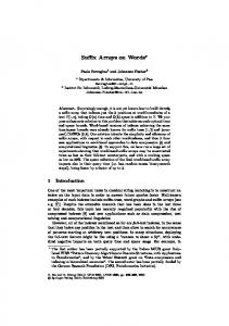
100MB for our experiments. The experiments were run on a Pentium IV, 2.0 GHz with 2GB RAM using Linux with kernel 2.4.31 and g++ with -O3 optimization. Compression performance. In Section 2.2 we mentioned that the compression time of exact Re-Pair would be an issue, and gave two approximate methods based on Ψ which should be faster. In this section we call RP our implementation of the exact Re-Pair compression algorithm6 , RPΨ0 the Ψ-based approximation that runs in O(n) time (Section 2.2), and RPΨ the Ψ-based approximation that runs in O(n log n) time (Section 2.3). We also include the methods RPSP, RPΨ0 SP, and RPΨSP. These forbid a rule to cross a 256-cell boundary. In all cases, we take absolute A′ samples each 64 positions. In practice, RPΨ0 and RPΨ0 SP are very fast in comparison with the rest of the methods, yet compress less. Considering this, we could relax the stopping condition with the aim of better balancing these factors. In Figure 3 we show space reduction achieved from one pass to the next, using RPΨ0 SP. For example, in the case of xml (the one needing the most passes), we remove 45% of the file in the first pass, and 40% of that in the second, but after 8 passes the compression gain is less than 0.01%. Considering this, we force at least 8 passes after reaching less than αn′ replacements per pass. We use α = 1/4, which gives good results.

Compression per pass, as percent

Compression per pass 50

xml english dna

40 30 20 10 0 0

Fig. 3.

2

4 6 Pass Number

8

10

Compression achived per pass using RPΨ0 SP. We use files of size 100MB.

To tune the parameters of the approximate variant RPΨSP, we test different values on two small files (english and xml, truncated to 50MB). We show, among several we carried out, the following experiments, as they best reflect the choice of parameters. Table I shows that the compression gain for increasing s loses importance for s > 8. Table II, on the other hand, shows that increasing δ does not give any gain on english, yet it slightly improves compression ratio on xml. A fair choice of parameters for RPΨSP, which we use for the rest of the experiments, is s = 8, δ = 3/4 and γ = log n. Table III shows that the compression ratio varies widely. On xml data we achieve 23.5% compression (the reduced suffix array is smaller than the text!), whereas compression is extremely poor on dna. In many text types of interest we slash the 6 Those

we could find freely available did not work properly. ACM Journal Name, Vol. V, No. N, Month 20YY.

16

· s 1 2 4 8 16 32 64 128

Compr. ratio xml 26.03% 25.95% 25.91% 25.89% 25.88% 25.87% 25.87% 25.87%

Compr. ratio english 55.47% 55.35% 55.32% 55.30% 55.29% 55.28% 55.28% 55.28%

Compr. time (sec) xml 766 905 1,080 1,241 1,344 1,519 1,645 1,717

Compr. time (sec) english 1,374 1,475 1,621 1,837 2,028 2,425 2,801 3,213

Table I. Compression ratio obtained using different values of s for the approximation RPΨSP. In this case we use δ = 1/2. The percentage is computed by comparing with the 4n bytes required by a standard suffix array implementation. δ 1/2 3/4 7/8 15/16 31/32

Compr. ratio xml 25.89% 25.81% 25.74% 25.68% 25.60%

Compr. ratio english 55.30% 55.29% 55.29% 55.29% 55.29%

Compr. time (sec) xml 1,241 1,573 2,091 2,835 4,185

Compr. time (sec) english 1,837 2,159 2,786 4,184 7,150

Table II. Compression obtained using different values of δ using approximation RPΨSP. In this case we use s = 8.

suffix array to around half of its size. Below the name of each collection we wrote the percentage H3 /H0 , which gives an idea of the compressibility of the collection independent of its alphabet size (e.g. it is very easy to compress dna to 25% because there are mainly 4 symbols but one chooses to spend a byte for each symbol in the uncompressed text, otherwise dna is almost incompressible). The measure turns out to be an excellent predictor of the compression, except for proteins where we are closer to H5 /H0 . We exclude dna to state the following numbers, because of its poor compression ratio. The approximation RPΨ0 runs up to 180 times faster and just loses 3.3%– 17.8% in compression ratio compared to RP. The approximation RPΨ runs up to 25 times faster and just loses up to 3.5% in compression ratio. RP runs at 25 to 1000 sec/MB, RPΨ0 runs at 5 to 10 sec/MB and RPΨ runs at 31 to 56 sec/MB. Suffix array construction is the same in all the methods and takes around 100 seconds overall in all cases. Thus, most of the indexing time shown in Table III is spent by the compression methods. Other statistics are also available in Table III. In column 6 we measure the average length of a cell of C if we choose uniformly in A (longer cells are in addition more likely to be chosen for decompression). Those numbers explain the times obtained for the next series of experiments. Note that they are related to compressibility, but not as much as one could expect. Rather, the numbers obey to a more detailed structure of the suffix array: they are higher when the compression is not uniform across the array. In every case, we can limit the maximum length of a C cell. The SP variants show how this impacts compression ratio and decompression speed. We can see that their compression ratio is almost the same, worsening at most by 6.37% (RP), 12.68% (RPΨ0 ), or 9.17% (RPΨ) on dna (and much less on others). ACM Journal Name, Vol. V, No. N, Month 20YY.

· Coll. size (MB),H3 /H0 xml,100, 26.28%

dna,100, 97.02%

english,100, 53.05%

pitches,50, 61.37%

proteins,100, 97.21%

sources,100, 40.74%

Method RP RPSP RPΨ0 RPΨ0 SP RPΨ RPΨSP RP RPSP RPΨ0 RPΨ0 SP RPΨ RPΨSP RP RPSP RPΨ0 RPΨ0 SP RPΨ RPΨSP RP RPSP RPΨ0 RPΨ0 SP RPΨ RPΨSP RP RPSP RPΨ0 RPΨ0 SP RPΨ RPΨSP RP RPSP RPΨ0 RPΨ0 SP RPΨ RPΨSP

Index size (MB) 93.56 99.52 103.06 116.13 94.26 102.90 336.53 337.11 342.52 343.11 336.37 336.96 227.59 230.04 249.03 252.08 227.74 230.26 116.58 117.61 126.56 127.83 117.98 119.18 284.61 285.94 294.08 296.24 285.94 287.73 154.88 159.34 181.38 187.52 156.18 161.21

Compr. ratio 23.39% 24.88% 25.76% 29.03% 23.56% 25.73% 84.13% 84.28% 85.63% 85.78% 84.09% 84.24% 56.90% 57.51% 62.26% 63.02% 56.94% 57.56% 58.29% 58.81% 63.28% 63.91% 58.99% 59.59% 71.15% 71.48% 73.52% 74.06% 71.49% 71.93% 38.72% 39.83% 45.34% 46.88% 39.04% 40.30%

Compr. time (s) 29,800 25,472 625 651 3,547 3,598 8,511 8,402 931 899 4,279 4,260 87,285 86,273 974 944 4,621 4,600 11,454 11,067 279 535 1,618 1,807 2,642 2,732 1,045 1,032 5,719 5,764 107,371 103,292 684 677 4,380 4,778

Expected decompr. 6,936.54 134.91 7,570.49 83.79 6,948.85 95.83 5.01 4.25 4.73 4.04 5.03 4.28 238.31 30.37 202.79 26.83 215.12 29.99 33.96 17.00 26.38 14.21 28.89 15.66 58.98 13.87 52.52 10.79 58.46 11.92 2,041.88 60.48 1,778.79 50.97 1,928.86 56.89

Dict. compr. 57.22% 58.29% 57.46% 58.68% 57.18% 58.23% 79.49% 79.72% 78.20% 78.44% 79.19% 79.41% 59.27% 59.71% 59.70% 60.19% 59.17% 59.60% 69.51% 70.08% 66.86% 67.23% 68.67% 69.00% 79.72% 80.09% 75.16% 75.03% 78.98% 78.80% 57.63% 58.33% 58.09% 58.80% 57.48% 58.13%

17

Compr. 2% in RAM 34.08% 35.84% 91.42% 91.59% 36.15% 40.63% 92.45% 92.56% 99.17% 99.18% 93.19% 93.30% 88.15% 88.33% 98.56% 98.56% 88.92% 89.12% 67.41% 67.78% 97.32% 97.34% 70.17% 71.03% 75.63% 76.00% 92.13% 92.30% 76.77% 77.31% 65.16% 65.85% 96.67% 96.70% 68.00% 69.15%

Table III. Index size and build time using Re-Pair and its Ψ-based approximations. We also include versions with rules up to length 256 (SP extension). Compression ratio compares with the 4n bytes needed by a plain suffix array representation.

In column 7 we show the compression ratio achieved on the dictionary part using the technique of Section 2.4, charging it the bitmap introduced as well. It can be seen that the technique is rather effective, approaching in some cases the limit of 50% to its possible effectiveness. (We remark that the compression ratios of previous columns do account for the dictionary space and all the necessary structures to operate.) The last column shows how much compression we would achieve if the structures that must reside on RAM were limited to 2% of the original suffix array size (recall Section 4.3). We still obtain attractive compression performance on texts like xml, sources and pitches (recall that on secondary memory the compression ratio translates almost directly to decompression performance). As expected, RPΨ0 does a much poorer job here, as it does not choose the best pairs early, but RPΨ achieves almost the same performance as RP. A classical reduced index. We test RPΨSP (from now on LCSA) as a replacement of the suffix array, that is, adding it the text and using it for binary searching, as explained in Section 4.1. We compare it with a plain suffix array (SA) and ACM Journal Name, Vol. V, No. N, Month 20YY.

·

18

M¨ akinen’s CSA (MakCSA [Mäkinen 2003]), as the latter operates similarly. Fig. 4 shows the result. MakCSA offers space-time tradeoffs, whereas those of our index (sample rate for absolute values) did not significantly affect the time. Our structure stands out as a relevant space/time tradeoff, especially when locating many occurrences (i.e., on short patterns). In particular, LCSA is usually noticeably faster than MakCSA for the same space, yet the latter is able of using less space (at least on english). Compared to a plain suffix array, LCSA requires 0.9–2.4 times the text size (as opposed to 4) plus the text, at the price of being 2–28 times slower for locating. Compared to current state of the art in compressed indexing, this slowdown is rather modest. Locate over english 0.6

0.3

0.5

Time(sec per 106 loc)


Locate over xml 0.35

0.25 0.2 0.15 0.1 0.05 0

0.4 0.3 0.2 0.1 0

0

0.5

1

1.5 2 2.5 3 IndexSize/TextSize-1

3.5

4

0

0.5

1

Locate over proteins



0.6 0.5 0.4 0.3 0.2 0.1 0 0.5

1


3.5

4

3.5

4

Locate over sources

0.7

0


3.5

4

0.5 0.45 0.4 0.35 0.3 0.25 0.2 0.15

LCSA m=05 MakCSA m=05 SA m=05 LCSA m=10 MakCSA m=10 SA m=10 LCSA m=15 MakCSA m=15 SA m=15

0.1 0.05 0 0

0.5

1


Fig. 4. Simulating a classical suffix array to binary search and locate the occurrences. Each file is of size 100MB.

A plugin for self-indexes. Section 4.2 considers using our reduced suffix array as a plugin to provide fast locate on existing self-indexes. In this experiment we plug our structure to the counting structures of the alphabet-friendly FM-index (AFI [Ferragina et al. 2007]), and compare the result against the original AFI, Sadakane’s CSA [Sadakane 2003] and the SSA [Ferragina et al. 2007; M¨ akinen and Navarro 2005], all from PizzaChili. We increased the sampling rate of the locating structures of AFI, CSA and SSA, to match the size of our LCSA. Fig. 5 shows the results. We only show four texts, as the others yield similar conclusions. The experiment consists in choosing random ranges of the suffix array and obtaining the values. This simulates a locating query where we can control ACM Journal Name, Vol. V, No. N, Month 20YY.

·

19

the amount of occurrences to locate. Our reduced suffix array has a constant time overhead (which is related to column 6 in Table III and the sample rate of absolute values) and from then on the cost per cell located is very low. As a consequence, it crosses sooner or later all the other indexes. For example, it becomes the fastest on xml after locating 2 occurrences, and after 8 occurrences it becomes the fastest on proteins. Particularly on xml, this success owes to the fact that our LCSA uses the RPΨSP variant (cutting phrases at length 256 as explained). If instead we used RPΨ to gain a little further compression, the result would be very inefficient due to the long phrases that need to be uncompressed. In the case of xml, RPΨ becomes the fastest only after locating 3,800 occurrences, not 2. In other texts where compression is not so good, there is not much difference between RPΨ and RPΨSP (both in time and space). Extract over xml

Extract over english 0.9 time(sec per 104 extractions)

time(sec per 104 extractions)

1.8 1.6 1.4 1.2 1 0.8 0.6 0.4 0.2 0

0.8 0.7 0.6 0.5 0.4 0.3 0.2 0.1 0

0

5

10 Extracted Size

15

20

0

5

Extract over proteins time(sec per 104 extractions)

time(sec per 104 extractions)

0.6 0.5 0.4 0.3 0.2 0.1 0 5

10 Extracted Size

15

20

15

20

Extract over sources

0.7

0

10 Extracted Size

15

20

1 0.9 0.8 0.7 0.6 0.5 0.4 0.3 0.2 0.1 0

LCSA SSA AF-index CSA

0

5

10 Extracted Size

Fig. 5. Time to locate occurrences, as a function of the number of occurrences to locate. Each file is of size 100MB.

6. LCSA CONSTRUCTION IN SECONDARY MEMORY Particularly for the application described in Section 4.3, where the LCSA does not fit in main memory, a natural question is whether is it possible to efficiently build it in secondary memory. Secondary memory algorithms to build the suffix array A are well-known [K¨ arkk¨ ainen and Rao 2003; Crauser and Ferragina 2002; Dementiev et al. 2005], yet the algorithms we have presented in Section 2 for compressing A′ are highly non-local. We now show that the algorithms to compress A′ by using ACM Journal Name, Vol. V, No. N, Month 20YY.

20

·

Ψ can be adapted efficiently to secondary memory, and also how to compress the dictionary in secondary memory. 6.1 Compressing the Differential Suffix Array When we compress in main memory by using Ψ (Sections 2.2 and 2.3), we notice that Ψ traverses the suffix array in increasing values of A[· ]. That is, if j is the position where A[j] = 1, then A[Ψ[j]] = 2, A[Ψ[Ψ[j]]] = 3 and so on. The idea is to store for each position i of A′ the information that permits us to compress A′ [i] after we sort it by increasing values of A, that is, by text order. For each position in A′ we define: —A′ [i] = A[i] − A[i − 1], 1 < i ≤ n; A′ [1] = A[1]. This is the differential form of A. —A′′ [i] = A′ [i + 1], 1 < i < n; A′′ [n] = ⊥ denotes an invalid value. —V ′ [i] = A[i], 1 ≤ i ≤ n. We will use this array to sort the rest. —N V ′ [i] = A[i + 1], 1 ≤ i < n; N V ′ [n] = ⊥. This is the position of the next valid symbol of A′ [i] after sorting. —N 2 V ′ [i] = A[i + 2], 1 ≤ i < n − 1; N V ′ [n − 1] = N V ′ [n] = ⊥. This is the position of the next-next valid symbol of A′ [i] after sorting. —P V ′ [i] = A[i − 1], 1 < i ≤ n; P V ′ [1] = ⊥, the position of the previous valid symbol of A′ [i] after sorting. Now we sort {A′ [i], A′′ [i], V ′ [i], N V ′ [i], N 2 V ′ [i], P V ′ [i]}1≤i≤n by the values of V = A. Given that A is a permutation of {1, . . . , n}, the effect of the sorting is that of composing the arrays with A−1 . We call the reordered arrays as follows: ′

—A˜′ [j] = A′ [A−1 [j]] = A[A−1 [j]] − A[A−1 [j] − 1], 1 ≤ j ≤ n, j 6= A[1]; A˜′ [A[1]] = A[1]. —A˜′′ [j] = A′′ [A−1 [j]] = A[A−1 [j] + 1] − A[A−1 [j]], 1 ≤ j ≤ n, j 6= A[n]; A˜′′ [A[n]] = ⊥. —V [j] = V ′ [A−1 [j]] = A[A−1 [j]] = j, 1 ≤ j ≤ n. —N V [j] = N V ′ [A−1 [j]] = A[A−1 [j] + 1], 1 ≤ j ≤ n, j 6= A[n]; N V [A[n]] = ⊥. —N 2 V [j] = N 2 V ′ [A−1 [j]] = A[A−1 [j] + 2], 1 ≤ j ≤ n, j 6= A[n], j 6= A[n − 1]; N V [A[n − 1]] = N V [A[n]] = ⊥. —P V [j] = P V ′ [A−1 [j]] = A[A−1 [j] − 1], 1 ≤ j ≤ n, j 6= A[1]; P V [A[1]] = ⊥. Now that we have the arrays {V [j], A˜′ [j], A˜′′ [j], N V [j], N 2 V [j], P V [j]}1≤j≤n , the sequential traversal of these arrays is equivalent to navigating the original ones using Ψ. More precisely, let j = A[i] (and thus i = A−1 [j]), then A˜′ [j] = A′ [i] and A˜′′ [j] = A′′ [i] = A′ [i+1]. Moreover, A˜′ [j+1] = A′ [Ψ(i)] and A˜′′ [j+1] = A′ [Ψ(i)+1]. Hence the check for pair equality between A′ [i]A′ [i + 1] and A′ [Ψ(i)]A′ [Ψ(i) + 1] reduces to checking whether A˜′ [j]A˜′′ [j] = A˜′ [j + 1]A˜′′ [j + 1], which can be carried out sequentially on A˜′ and A˜′′ . The other arrays are used to maintain consistency upon changes in A′ : When we change A˜′ [j] and A˜′′ [j], corresponding to A′ [i] and A′ [i + 1], we have the problem that the pair A′ [i − 1]A′ [i], which is explicitly stored at A˜′ [P V [j]] and A˜′′ [P V [j]], must be updated as well. Similarly, N V serves to locate the place where the pair corresponding to A′ [i + 1]A′ [i + 2] is stored after the sorting. Thus, as the arrays ACM Journal Name, Vol. V, No. N, Month 20YY.

·

21

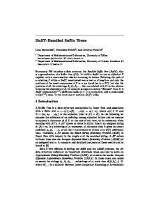
are now sorted by j = A[i], arrays P V and N V serve as a doubly-linked list to let us move to i − 1 and i + 1 in the sorted array. Those lists must be updated upon removals across the compression process, and they are also useful to maintain the current values of A˜′′ [j] up to date when elements in the chain are removed. Let τ be the total size in integers of these arrays. We divide them into l chunks of size τ /l and, for each chunk, we keep in main memory a buffer of ˜b integers. Let M be the size in integers of the main memory, then τ /l + l· ˜b ≤ M must hold (we consider later the case where M is smaller). The algorithm to carry out a single pass on A′ in secondary memory is as follows. Note that this is the main subroutine of both approximate methods based on Ψ (Sections 2.2 and 2.3). (1) We read the first chunk from disk and initialize empty buffers. (2) We find sequentially in the chunk the first j satisfying A˜′ [j]A˜′′ [j] = A˜′ [j + 1]A˜′′ [j + 1]. If no such j is found we go on with the next chunk. In the stronger approximate method we require equality between several A˜′ [j +r]A˜′′ [j +r] pairs before proceeding to the next step. (3) From that j, we start a chain of replacements: We add a new pair s ← A˜′ [j]A˜′′ [j] to R, make the replacements at j and j + 1 and move on with j ← j + 1, replacing until the pair changes. When the pair changes, that is A˜′ [j]A˜′′ [j] 6= A˜′ [j + 1]A˜′′ [j + 1], we restart the search for pairs at Step (2). (4) If we reach the end of the block, the replacement chain may continue at the next one. To consistently perform a replacement A˜′ [j] : A˜′′ [j] ← s : ⊥ in Step (3), maintaining also the linked lists, we must carry out the following actions (in parallel; we overline variables to indicate that we use their original values prior to any assignment): (a) A˜′ [j] ← s, (b) A˜′ [N V [j]] ← ⊥, (c) A˜′′ [j] ← A˜′′ [N V [j]], (d) N V [j] ← N 2 V [j], (e) P V [N 2 V [j]] ← j, (f ) N 2 V [j] ← N 2 V [N V [j]], (g) A˜′′ [P V [j]] ← s, and (h) N 2 V [P V [j]] ← N 2 V [j]. From those, only (a) and (d) can be executed locally, whereas the others may require reading/writing data from/to other chunks not yet in main memory. If this is the case, we “send messages” to read/update other chunks. Those will be stored in their corresponding buffers, and carried out right before those chunks are processed. (If a buffer gets full it is written out to disk into a log of actions the chunk must execute.) Some of those messages will then send messages back to the current chunk to update its values, and this update will be executed when the current chunk is read again. This is not a problem because we will not access cell j again until the next pass. (The updates that happen to belong to the current chunk, instead, must be executed immediately.) Each message is of the form action(dest, parameters), where dest is the destination position that determines the chunk ⌈dest/l⌉ that will execute it; see Table IV for the meaning of each action. The global instructions we described are then translated into the following instructions and messages sent: (a) A˜′ [j] ← s, (b) send DL(N V [j], j) (will solve (c) and (f ) in the next pass), (d) N V [j] ← N 2 V [j], (e) send U P (N 2 V [j], j), (g) send U A′′ (P V [j], s), and (h) send U N 2 (P V [j], N 2 V [j]). Figure 6 shows the operations that are performed after a replacement; this occurs in three steps. Thus, at the end of the pass, we must carry out two extra passes in order to process the messages sent and their responses, before finishing the pass ACM Journal Name, Vol. V, No. N, Month 20YY.

·

22

(g) U A′′ (P V [j], s)

(I)

(b,c,f) DL(N V [j], j) N V [j]

j

P V [j] A˜′ A˜′′

N 2 V [j]

s ← (a)

PV N 2 V [j]

NV

(d)

N 2V (h) U N 2 (P V [j], N 2 V [j]) (II)

j

P V [j] A˜′ A˜′′

(e) U P (N 2 V [j], j) (c) U A′′ (j, A˜′′ [N V [j]]) N V [j]

s ← (a)

⊥ ← (b)

s ← (g) (e) → j

PV N 2 V [j] ← (d)

NV N 2V

N 2 V [j]

N 2 V [j] ← (h) (f) U N 2 (j, N 2 V [N V [j]])

(III)

j

P V [j] A˜′ A˜′′

s ← (a)

⊥ ← (b)

A˜′′ [N V [j]] ← (c)

s ← (g)

(e) → j

PV N 2 V [j] ← (d)

NV N 2V

N 2 V [j]

N V [j]

N 2 V [j] ← (h)

N 2 V [N V [j]] ← (f)

Fig. 6. Operations generated by a replacement. (I) shows the replacement and the messages generated by it. (II) shows the effect of the messages, one of which generates two more messages. (III) shows the final state product of a replacement.

properly. action U A′ U A′′ UN2 DL UP Table IV.

parameter sym sym next f rom prev

what it does at position dest ˜′ to sym, A ˜′ [dest] ← sym. Updates A ˜′′ to sym, A ˜′′ [dest] ← sym. Updates A Updates N 2 V to next, N 2 V [dest] ← next. Marks dest as deleted and responds with ˜′′ [dest]) and U N 2 (f rom, N 2 V [dest]) U A′′ (f rom, A Updates P V to prev, P V [dest] ← prev.

Message types and meanings used by the secondary memory construction algorithm.

The invalid entries we produce must be compacted for the next passes. Apart from removing the invalid entries, we must update the pointers N V , N 2 V , and P V . We first sort all the arrays by the N V values. The result will be an increasing sequence of N V [i] values, with some missing integers due to the removed entries. Thus we assign N V [i] ← i to effectively remove the invalid entries. We repeat the ACM Journal Name, Vol. V, No. N, Month 20YY.

·

23

process of sorting and reassigning for N 2 V and P V . Finally we sort again by V , and are ready for the next pass. Thus, each pass of the original algorithm over an array of size n′ costs us, in I/O terms, O(n′ /˜b) for the traversal plus O((n′ /˜b) logM/˜b (n′ /M )) = O(Sort(n′ )) for the sortings. It is easy to see that, because the n′ s are of the form (1 − α)i n, the linear-time algorithm of Section 2.2 costs O(Sort(n)) in secondary memory. Similarly, the O(n log n) time algorithm of Section 2.3 costs O(Sort(n) log n) time. This is almost I/O optimal with respect to the original algorithms. As a practical note, Figure 3 shows that indeed 8 passes are sufficient, even on xml, to achieve most of the compression on the variants we tried. With respect to the extra secondary memory needed, it is O(n) words for the arrays, plus the message logs. Since each position can receive O(1) messages from elsewhere, all the message logs add up to O(n) words as well. Finally, we consider the case τ /l + l· ˜b > M , that is, there is no space to store one disk page per chunk in main memory. In this case we replace the in-memory buffers by a secondary-memory priority queue, where the messages are inserted with priority given by dest. Those sent from a chunk i to a position dest < i will be inserted with priority n + dest, so that they are processed in a second traversal. Each new chunk reads from the priority queue (by means of extracting minima) all the messages that correspond to it, and inserts new messages. As there are overall O(n) messages, optimal-I/O priority queues (e.g. [Brengel et al. 2000]) yield O((n′ /˜b) logM/˜b (n′ /˜b)) overall time, which raises only slightly the O(Sort(n′ )) time per pass we had. 6.2 Compressing the Dictionary When we compress the dictionary in main memory, we start expanding the first (i.e. earliest) rule sj that has not been used by another one, U [j] = 0 (see Section 2.4). Then we expand the next rule sj ′ that has U [j ′ ] = 0, and so on. The idea here is to group together all the rules that are used in the same expansion of a rule with value U [·] = 0, so that when we expand it we will have almost all the information needed to do the expansion in main memory. We can regard the dictionary as R = {s1 → a1 b1 , s2 → a2 b2 , . . . , sν → aν bν }, where si = i + n. For each rule we define: —R0 [i] = si , the value of the i-th rule. —R1 [i] = ai , the left symbol of the i-th rule. It can be a rule or an original symbol. —R2 [i] = bi , the right symbol of the i-th rule. It can be a rule or an original symbol. min{sj , si is used by sj ∧ U [j] = 0} if U [i] = 1, —Q[i] = si otherwise. The min is the lowest (i.e. earliest) rule that contains si and has value U [·] = 0. Rules with the same value of Q will be used in the same expansion, so Q will be a kind of group identifier. Given the non-locality of reference between rules, to calculate the values of Q we need to send messages of the form U Q(dest, parameter), to achieve Q[dest] ← ACM Journal Name, Vol. V, No. N, Month 20YY.

24

·

parameter, with 1 ≤ dest, parameter ≤ ν. Note that a position dest could receive multiple messages and that always dest < parameter. We maintain a secondary-memory priority queue P Q, where the messages are inserted with priority given by dest (larger first). We process the arrays from higher values of R0 first, i.e., in reverse order. To process cell i we extract from P Q all the messages for dest = i and set Q[i] to the minimum parameter for that i. If there are no messages for i, we assign a new Q[i] ← si (i.e., we do not need to store U ). Then we insert message U Q(R1 [i], Q[j]) (U Q(R2 [i], Q[j])) into P Q, if R1 [i] (R2 [i]) is not an original symbol. Since any rule R0 [j] that uses rule R0 [i] has been visited before we reach position i, necessarily the message U Q(R0 [i], Q[j]) is in P Q by that time. Thus we compute array Q in one pass. Now we sort these arrays by increasing values of the pair (Q[i], R0 [i]), i.e., by Q ˜ R ˜0, R ˜1, R ˜ 2 . These arrays can be partitioned and using R0 to break ties, obtaining Q, into η groups, each one with the same value of Q. Let ηk be the position where the k-th group finishes. Note that if the length of the longest phrase is µ then any group has at most µ elements. Now, for each group, we compress the dictionary almost the same way as in algorithm Expand Rule (see Figure 2, page 10). There are four differences with the original algorithm: (1) We write down RB and RS to disk instead of maintaining them in main memory. The array N V is not used. ˜ 0 [ηk ], the last element of the k-th group, because by construction (2) We expand R these rules use all the other rules in the same group. ˜ 0 [i], which is expanded to R ˜ 1 [i]R ˜ 2 [i], we do as follows. If R ˜ 1 [i] (3) To process rule R ˜ is not an original symbol, and it does not belong to the same group of R0 [i], then it must have been defined in a previous group. Hence we must not expand it further, but instead write its final value in RS . Yet this value is only know ˜ 1 [i]), where pos is the within the other group. We send message N RS (pos, R ˜ 2 [i]. current position where we are writing in RS . The same goes for R (4) We also write down to disk the pair (sj , LRB [sj ]) (second line of algorithm Expand Rule), where sj is the rule and LRB [sj ] is its final value (i.e., the current value of variable LRB ). After carrying out the previous steps, we still need to execute the messages N RS to update RS . We sort the messages by dest (their first component) obtaining N RS = (dest, parameter), and sort the pairs (sj , LRB [sj ]) by its first coordinate, obtaining (sj , LRB ). Because the compressed dictionary will hold at least ν integers in RAM, we can use that RAM space across the process. From now on LRB will reside completely in main memory, so we can access it at random. To apply the messages we traverse N RS and RS making the necessary replacements in RS , that is, RS [dest[i]] = LRB [parameter[i]−n]. These replacements are done by increasing values of dest, so we traverse only once the arrays N RS and RS . Using again LRB we traverse C, changing the values of the rules to their final ones. Let M be the size in integers of the main memory. The breakdown of the cost is as follows: —When we calculate Q there are overall O(ν) messages. Using optimal-I/O priority queues (e.g. [Brengel et al. 2000]) yields O((ν/˜b) logM/˜b (ν/˜b)) time. ACM Journal Name, Vol. V, No. N, Month 20YY.

·

25

—When we expand a rule we need to find both children. Each such search within their group takes at most log µ CPU time. Overall there are at most 2ν of these searches, totalizing O(ν log µ) CPU time. —We take O(ν/˜b) I/Os to read/write all the needed arrays from disk. —There are three sortings, which in total take O(Sort(ν)) time. —Updating C to the new rule values takes O(n′ /˜b) I/Os . Overall, time is O((ν/˜b) log ˜(ν/˜b) + n′ /˜b) I/Os. The extra space on disk is M/b

O(ν) integers. Note that 4µ ≤ M must hold to be able to compress a group in main memory. If LRB does not fit in main memory, we pre-process the messages first, that is, we first sort N RS by parameter, then we traverse it in synchronization with LRB updating parameter ← LRB (parameter), and then we sort again N RS by dest. Now we only need to traverse RS and N RS together, to update RS . This add an extra O(Sort(ν)) time to the cost, which does not affect our complexity. Something similar can be done to update C, which incurs an extra cost of O(Sort(n′ )). This would affect the complexity, but is still within the cost paid in Section 6.1 to build C. 7. CONCLUSIONS AND FUTURE WORK We have presented a suffix array compression method that retains fast locating of the occurrences of a pattern. We have proved analytically that the resulting size is related to the k-th order entropy of the text. The method has been used to obtain a compressed self-index with fast locate (where the norm is to be extremely slow), a small index that is a viable alternative to classical suffix arrays, and a secondary-memory version that works optimally and whose access time improves due to compression (where worsening is the norm). Our experiments show that the structure is very practical and relevant. As a byproduct, we have presented Re-Pair algorithms tailored to suffix array differences, which exploit the structure of Ψ to run much faster and using much less memory than the general algorithm. Those new algorithms are approximations, yet we show that their compression loss is negligible. We also presented a secondary memory construction for those approximations, which run almost I/O-optimally and extends the applicability of the methods to compress suffix arrays that do not fit in main memory. Another byproduct, which might be of general interest, is a compact data structure to represent the Re-Pair dictionary. This structure can reduce the dictionary space by up to 50%, and operates in compressed form, that is, it permits decompressing parts of the text without uncompressing the dictionary. Our work leaves several future development lines. In the short term, we seek to improve the performance of the smaller classical index via algorithm engineering, and implement the secondary memory index, which is right now a theoretical proposal. In this latter line, we are working on merging the CPT structure presented by Clark and Munro [1996] with our structure. We believe the result would be extremely competitive in practice. In the longer term, we believe this is a first step towards compressed text indexes with competitive locating times, in particular via locality of access. The key was to ACM Journal Name, Vol. V, No. N, Month 20YY.

26

·

build on the runs in Ψ, which have been used in the past to achieve compression yet not locality of access. We showed that the regularities that Re-Pair exploits on the differential suffix array are closely related to those runs in Ψ. Thus we could take advantage of the locality properties of Re-Pair, and also used the close relation with Ψ to analyze the compression achieved and design faster Re-Pair variants for this case. Our resulting index is still far from achieving the space used by the smallest self-indexes, which are however extremely slow to locate. Is there a fundamental lower bound to the tradeoff one can achieve between space and time for locating? Is there a limit to what can be achieved via local compression? REFERENCES Baeza-Yates, R., Barbosa, E. F., and Ziviani, N. 1996. Hierarchies of indices for text searching. Information Systems 21, 6, 497–514. Brengel, K., Crauser, A., Ferragina, P., and Meyer, U. 2000. An experimental study of priority queues in external memory. ACM Journal of Experimental Algorithmics 5, 17. Clark, D. and Munro, I. 1996. Efficient suffix trees on secondary storage. In Proc. 7th SODA. 383–391. Crauser, A. and Ferragina, P. 2002. A theoretical and experimental study on the construction of suffix arrays in external memory. Algorithmica 32, 1, 1–35. ¨ rkka ¨ inen, J., Mehnert, J., and Sanders, P. 2005. Better external memory Dementiev, R., Ka suffix array construction. In Proc. 7th Workshop on Algorithm Engineering and Experiments (ALENEX) (2007-01-30). 86–97. Ferragina, P. and Grossi, R. 1999. The string B-tree: A new data structure for string search in external memory and its applications. Journal of the ACM 46, 2, 236–280. Ferragina, P. and Manzini, G. 2005. Indexing compressed texts. J. of the ACM 52, 4, 552–581. ¨ kinen, V., and Navarro, G. 2007. Compressed representations Ferragina, P., Manzini, G., Ma of sequences and full-text indexes. ACM Transactions on Algorithms (TALG) 3, 2, article 20. ´ lez, R. and Navarro, G. 2006. Statistical encoding of succinct data structures. In Proc. Gonza 17th CPM. LNCS 4009. 295–306. ´ lez, R. and Navarro, G. 2007. A compressed text index on secondary memory. In Proc. Gonza 18th IWOCA. College Publications, UK, 80–91. Grossi, R., Gupta, A., and Vitter, J. 2003. High-order entropy-compressed text indexes. In Proc. 14th SODA. 841–850. Grossi, R. and Vitter, J. 2006. Compressed suffix arrays and suffix trees with applications to text indexing and string matching. SIAM Journal on Computing 35, 2, 378–407. Jacobson, G. 1989. Space-efficient static trees and graphs. In Proc. 30th FOCS. 549–554. ¨ rkka ¨ inen, J. and Rao, S. 2003. Algorithms for Memory Hierarchies. LNCS v. 2625. Springer, Ka Chapter 7: Full-text indexes in external memory, 149–170. Larsson, J. and Moffat, A. 2000. Off-line dictionary-based compression. Proc. IEEE 88, 11, 1722–1732. ¨ kinen, V. 2003. Compact suffix array — a space-efficient full-text index. Fundamenta InforMa maticae 56, 1–2, 191–210. ¨ kinen, V. and Navarro, G. 2005. Succinct suffix arrays based on run-length encoding. Nordic Ma J. of Computing 12, 1, 40–66. ¨ kinen, V., Navarro, G., and Sadakane, K. 2004. Advantages of backward searching — Ma efficient secondary memory and distributed implementation of compressed suffix arrays. In Proc. 15th ISAAC. LNCS v. 3341. 681–692. Manber, U. and Myers, G. 1993. Suffix arrays: a new method for on-line string searches. SIAM J. Computing 22, 5, 935–948. Manzini, G. 2001. An analysis of the Burrows-Wheeler transform. J. of the ACM 48, 3, 407–430. Navarro, G. 2004. Indexing text using the Ziv-Lempel trie. J. of Discrete Algorithms 2, 1, 87–114. ACM Journal Name, Vol. V, No. N, Month 20YY.

·

27

¨ kinen, V. 2007. Compressed full-text indexes. ACM Computing SurNavarro, G. and Ma veys 39, 1, article 2. Sadakane, K. 2003. New text indexing functionalities of the compressed suffix arrays. J. of Algorithms 48, 2, 294–313. Weiner, P. 1973. Linear pattern matching algorithm. In Proc. 14th IEEE Symp. on Switching and Automata Theory. 1–11.

Received Month Year; revised Month Year; accepted Month Year.
