Faster Discovery of Faster System Configurations with Spectral Learning

Noname manuscript No. (will be inserted by the editor)

Faster Discovery of Faster System Configurations with Spectral Learning Vivek Nair · Tim Menzies · Norbert Siegmund · Sven Apel

arXiv:1701.08106v1 [cs.SE] 27 Jan 2017

Received: date / Accepted: date

Abstract Despite the huge spread and economical importance of configurable software systems, there is unsatisfactory support in utilizing the full potential of these systems with respect to finding performance-optimal configurations. Prior work on predicting the performance of software configurations suffered from either (a) requiring far too many sample configurations or (b) large variances in their predictions. Both these problems can be avoided using the WHAT spectral learner. WHAT’s innovation is the use of the spectrum (eigenvalues) of the distance matrix between the configurations of a configurable software system, to perform dimensionality reduction. Within that reduced configuration space, many closely associated configurations can be studied by executing only a few sample configurations. For the subject systems studied here, a few dozen samples yield accurate and stable predictors—less than 10 % prediction error, with a standard deviation of less than 2 %. When compared to the state of the art, WHAT (a) requires 2 to 10 times fewer samples to achieve similar prediction accuracies, and (b) its predictions are more stable (i.e., have lower standard deviation). Furthermore, we demonstrate that predictive models generated by WHAT can be used by optimizers to discover system configurations that closely approach the optimal performance. Keywords Performance Prediction · Spectral Learning · Decision Trees · SearchBased Software Engineering · Sampling. Vivek Nair North Carolina State University, Raleigh, USA E-mail: [email protected] Tim Menzies North Carolina State University, Raleigh, USA E-mail: [email protected] Norbert Siegmund University of Weimar, Germany E-mail: [email protected] Sven Apel University of Passau, Germany E-mail: [email protected]

2

Vivek Nair et al.

1 Introduction Most software systems today are configurable. Despite the undeniable benefits of configurability, large configuration spaces challenge developers, maintainers, and users. In the face of hundreds of configuration options, it is difficult to keep track of the effects of individual configuration options and their mutual interactions. So, predicting the performance of individual system configurations or determining the optimal configuration is often more guess work than engineering. In their recent paper, Xu et al. documented the difficulties developers face with understanding the configuration spaces of their systems [40]. As a result, developers tend to ignore over 5/6ths of the configuration options, which leaves considerable optimization potential untapped and induces major economic cost [40]. Addressing the challenge of performance prediction and optimization in the face of large configuration spaces, researchers have developed a number of approaches that rely on sampling and machine learning [15, 29, 35]. While gaining some ground, state-of-the-art approaches face two problems: (a) they require far too many sample configurations for learning or (b) they are prone to large variances in their predictions. For example, prior work on predicting performance scores using regression trees had to compile and execute hundreds to thousands of specific system configurations [15]. A more balanced approach by Siegmund et al. is able to learn predictors for configurable systems [35] with low mean errors, but with large variances of prediction accuracy (e.g. in half of the results, the performance predictions for the Apache Web server were up to 50 % wrong). Guo et al. [15] also proposed an incremental method to build a predictor model, which uses incremental random samples with steps equal to the number of configuration options (features) of the system. This approach also suffered from unstable predictions (e.g., predictions had a mean error of up to 22 %, with a standard deviation of up 46 %). Finally, Sarkar et al. [29] proposed a projective-learning approach (using fewer measurements than Guo at al. and Siegmund et al.) to quickly compute the number of sample configurations for learning a stable predictor. However, as we will discuss, after making that prediction, the total number of samples required for learning the predictor is comparatively high (up to hundreds of samples). The problems of large sample sets and large variances in prediction can be avoided using the WHAT spectral learner, which is our main contribution. WHAT’s innovation is the use of the spectrum (eigenvalues) of the distance matrix between the configurations of a configurable system, to perform dimensionality reduction. Within that reduced configuration space, many closely associated configurations can be studied by measuring only a few samples. In a number of experiments, we compared WHAT against the state-of-the-art approaches of Siegmund et al. [35], Guo et al. [15], and Sarkar et al. [29] by means of six real-world configurable systems: Berkeley DB, the Apache Web server, SQLite, the LLVM compiler, and the x264 video encoder. We found that WHAT performs as well or better than prior approaches, while requiring far fewer samples (just a few dozen). This is significant and most surprising, since some of the systems explored here have up to millions of possible configurations.

Faster Discovery of Faster System Configurations with Spectral Learning

3

Overall, we make the following contributions: – We present a novel sampling and learning approach for predicting the performance of software configurations in the face of large configuration spaces. The approach is based on a spectral learner that uses an approximation to the first principal component of the configuration space to recursively cluster it, relying only on a few points as representatives of each cluster. – We demonstrate the practicality and generality of our approach by conducting experiments on six real-world configurable software systems (see Figure 1). The results show that our approach is more accurate (lower mean error) and more stable (lower standard deviation) than state-of-the-art approaches. A key finding is the utility of the principal component of a configuration space to find informative samples from a large configuration space. All materials required for reproducing this work are available at https:// goo.gl/689Dve.

2 Background & Related Work A configurable software system has a set X of Boolean configuration options,1 also referred to as features or independent variables in our setting. We denote the number of features of system S as n. The configuration space of S can be represented by a Boolean space Zn2 , which is denoted by F. All valid configurations of S belong to a set V , which is represented by vectors Ci (with 1 ≤ i ≤ |V |) in Zn2 . Each element of a configuration represents a feature, which can either be True or False, based on whether the feature is selected or not. Each valid instance of a vector (i.e., a configuration) has a corresponding performance score associated to it. The literature offers two approaches to performance prediction of software configurations: a maximal sampling and a minimal sampling approach: With maximal sampling, we compile all possible configurations and record the associated performance scores. Maximal sampling can be impractically slow. For example, the performance data used in our experiments required 26 days of CPU time for measuring (and much longer, if we also count the time required for compiling the code prior to execution). Other researchers have commented that, in real world scenarios, the cost of acquiring the optimal configuration is overly expensive and time consuming [39]. If collecting performance scores of all configurations is impractical, minimal sampling can be used to intelligently select and execute just enough configurations (i.e., samples) to build a predictive model. For example, Zhang et al. [42] approximate the configuration space as a Fourier series, after which they can derive an expression showing how many configurations must be studied to build predictive models with a given error. While a theoretically satisfying result, that approach still needs thousands to hundreds of thousands of executions of sample configurations. Another set of approaches are the four ”additive” minimal sampling methods of Siegmund et al. [35]. Their first method, called feature-wise sampling (FW), is their 1 In this paper, we concentrate on Boolean options, as they make up the majority of all options; see Siegmund et al., for how to incorporate numeric options [34].

4

Vivek Nair et al.

basic method. To explain FW, we note that, from a configurable software system, it is theoretically possible to enumerate many or all of the valid configurations2 . Since each configuration (Ci ) is a vector of n Booleans, it is possible to use this information to isolate examples of how much each feature individually contributes to the total run time: 1. Find a pair of configurations C1 and C2 , where C2 uses exactly the same features as C1 , plus one extra feature fi . 2. Set the run time Π ( fi ) for feature fi to be the difference in the performance scores between C2 and C1 . 3. The run time for a new configuration Ci (with 1 ≤ i ≤ |V |) that has not been sampled before is then the sum of the run time of its features, as determined before: Π (Ci ) = ∑ Π ( f j ) (1) f j ∈Ci

When many pairs, such as C1 , C2 , satisfy the criteria of point 1, Siegmund et al. used the pair that covers the smallest number of features. Their minimal sampling method, FW, compiles and executes only these smallest C1 and C2 configurations. Siegmund et al. also offers three extensions to the basic method, which are based on sampling not just the smallest pairs, but also additional configurations covering certain kinds of interactions between features. All the following minimal sampling policies compile and execute valid configurations selected via one of three heuristics: PW (pair-wise): For each pair of features, try to find a configuration that contains the pair and has a minimal number of features selected. HO (higher-order): Select extra configurations, in which three features, f1 , f2 , f3 , are selected if two of the following pair-wise interactions exist: ( f1 , f2 ) and ( f2 , f3 ) and ( f1 , f3 ). HS (hot-spot): Select extra configurations that contain features that are frequently interacting with other features. Guo et al. [15] proposed a progressive random sampling approach, which samples the configuration space in steps of the number of features of the software system in question. They used the sampled configurations to train a regression tree, which is then used to predict the performance scores of other system configurations. The termination criterion of this approach is based on a heuristic, similar to the PW heuristics of Siegmund et al. Sarkar et al. [29] proposed a cost model for predicting the effort (or cost) required to generate an accurate predictive model. The user can use this model to decide whether to go ahead and build the predictive model. This method randomly samples configurations and uses a heuristic based on feature frequencies as termination criterion. The samples are then used to train a regression tree; the accuracy of the model is measured by using a test set (where the size of the training set is equal to size of the test set). One of four projective functions (e.g., exponential) is selected based on how 2 Though, in practice, this can be very difficult. For example, in models like the Linux Kernel such an enumeration is practically impossible [30].


5

correlated they are to accuracy measures. The projective function is used to approximate the accuracy-measure curve, and the elbow point of the curve is then used as the optimal sample size. Once the optimal size is known, Sarkar et al. uses the approach of Guo et al. to build the actual prediction model. The advantage of these previous approaches is that, unlike the results of Zhang et al., they require only dozens to hundreds of samples. Also, like our approach, they do not require to enumerate all configurations, which is important for highly configurable software systems. That said, as shown by our experiments (see Section 4), these approaches produce estimates with larger mean errors and partially larger variances than our approach. While sometimes the approach by Sarkar et al. results in models with (slightly) lower mean error rates, it still requires a considerably larger number of samples (up to hundreds), while WHAT requires only few dozen.

3 Approach 3.1 Spectral Learning The minimal sampling method we propose here is based on a spectral-learning algorithm that explores the spectrum (eigenvalues) of the distance matrix between configurations in the configuration space. In theory, such spectral learners are an appropriate method to handle noisy, redundant, and tightly inter-connected variables, for the following reasons: When data sets have many irrelevancies or closely associated data parameters d, then only a few eigenvectors e, e d are required to characterize the data. In this reduced space: – Multiple inter-connected variables i, j, k ⊆ d can be represented by a single eigenvector; – Noisy variables from d are ignored, because they do not contribute to the signal in the data; – Variables become (approximately) parallel lines in e space. For redundancies i, j ∈ d, we can ignore j since effects that change over j also change in the same way over i; That is, in theory, samples of configurations drawn via an eigenspace sampling method would not get confused by noisy, redundant, or tightly inter-connected variables. Accordingly, we expect predictions built from that sample to have lower mean errors and lower variances on that error. Spectral methods have been used before for a variety of data mining applications [20]. Algorithms, such as PDDP [4], use spectral methods, such as principle component analysis (PCA), to recursively divide data into smaller regions. Softwareanalytics researchers use spectral methods (again, PCA) as a pre-processor prior to data mining to reduce noise in software-related data sets [37]. However, to the best of our knowledge, spectral methods have not been used before as a basis of a minimal sampling method. WHAT is somewhat different from other spectral learners explored in, for instance, image processing applications [31]. Work on image processing does not aim

6

Vivek Nair et al.

at defining a minimal sampling policy to predict performance scores. Also, a standard spectral method requires an O(N 2 ) matrix multiplication to compute the components of PCA [18]. Worse, in the case of hierarchical division methods, such as PDDP, the polynomial-time inference must be repeated at every level of the hierarchy. Competitive results can be achieved using an O(2N) analysis that we have developed previously [24], which is based on a heuristic proposed by Faloutsos and Lin [10] (which Platt has shown computes a Nystr¨om approximation to the first component of PCA [27]). WHAT receives N (with 1 ≤ |N| ≤ |V |) valid configurations (C), N1 , N2 , ..., as input and then: 1. Picks any point Ni (1 ≤ i ≤ |N|) at random; 2. Finds the point West ∈ N that is furthest away from Ni ; 3. Finds the point East ∈ N that is furthest from West. The line joining East and West is our approximation for the first principal component. Using the distance calculation shown in Equation 2, we define δ to be the distance between East (x) and West (y). WHAT uses this distance (δ ) to divide all the configurations as follows: The value xi is the projection of Ni on the line running from East to West3 . We divide the examples based on the median value of the projection of xi . Now, we have two clusters of data divided based on the projection values (of Ni ) on the line joining East and West. This process is applied recursively on these clusters until a predefined stopping condition. In our pstudy, the recursive splitting of the Ni ’s stops when a sub-region contains less than |N| examples. p 2  ( ∑i (xi − yi ) dist(x, y) = 0, if xi = yi   1, otherwise

if xi and yi is numeric if xi and yi is Boolean

(2)

We explore this approach for three reasons: – It is very fast: This process requires only 2|n| distance comparisons per level of recursion, which is far less than the O(N 2 ) required by PCA [8] or other algorithms such as K-Means [16]. – It is not domain-specific: Unlike traditional PCA, our approach is general in that it does not assume that all the variables are numeric. As shown in Equation 2,4 we can approximate distances for both numeric and non-numeric data (e.g., Boolean). – It reduces the dimensionality problem: This technique explores the underlying dimension (first principal component) without getting confused by noisy, related, and highly associated variables. 3

The projection of Ni can be calculatedqin the following way:

a = dist(East, Ni ); b = dist(West, Ni ); xi = 4

a2 −b2 +δ 2 2δ

.

In our study, dist accepts pair of configuration (C) and returns the distance between them. If xi and yi ∈ Rn , then the distance function would be same as the standard Euclidean distance.


7

3.2 Spectral Sampling When the above clustering method terminates, our sampling policy (which we call S1 ) is then applied: Random sampling (S1 ): compile and execute one configuration, picked at random, from each leaf cluster; We use this sampling policy, because (as we will show later) it performs better than: East-West sampling (S2 ): compile and execute the East and West poles of the leaf clusters; Exemplar sampling (S3 ): compile and execute all items in all leaves and return the one with lowest performance score. Note that S3 is not a minimal sampling policy (since it executes all configurations). We use it here as one baseline against which we can compare the other, more minimal, sampling policies. In the results that follow, we also compare our sampling methods against another baseline using information gathered after executing all configurations.

3.3 Regression-Tree Learning After collecting the data using one of the sampling policies (S1 , S2 , or S3 ), as described in Section 3.2, we use a CART regression-tree learner [5] to build a performance predictor. Regression-tree learners seek the attribute-range split that most increases our ability to make accurate predictions. CART explores splits that divide N samples into two sets A and B, where each set has a standard deviation on the target variable of σ1 and σ2 . CART finds the “best” split defined as the split that minimizes B A N σ1 + N σ2 . Using this best split, CART divides the data recursively. In summary, WHAT combines: – The FASTMAP method of Faloutsos and Lin [10], which rather than N 2 comparisons only performs 2N where N is the number of configurations in the configuration space; – A spectral-learning algorithm initially inspired by Boley’s PDDP system [4], which we modify by replacing PCA with FASTMAP (called “WHERE” in prior work [24]); – The sampling policy that explores the leaf clusters found by this recursive division; – The CART regression-tree learner that converts the data from the samples collected by sampling policy into a run-time prediction model [5]. That is, WHERE

=

PDDP − PCA + FASTMAP

WHAT

=

WHERE + { S1 , S2 , S3 } + CART

This unique combination of methods has not been previously explored in the softwareengineering literature.

8

Vivek Nair et al.

4 Experiments 4.1 Research Questions We formulate our research questions in terms of the challenges of exploring large complex configuration spaces. As our approach explores the spectral space, our hypothesis is that only a small number of samples is required to explore the whole space. However, a prediction model built from a very small sample of the configuration space might be very inaccurate and unstable, that is, it may exhibit very large mean prediction errors and variances on the prediction error. Also, if we learn models from small regions of the training data, it is possible that a learner will miss trends in the data between the sample points. Such trends are useful when building optimizers (i.e., systems that receives one configuration as input and propose an alternate configuration that has, for instance, a better performance). Such optimizers might need to evaluate hundreds to millions of alternate configurations. To speed up that process, optimizers can use a surrogate model 5 that mimics the outputs of a system of interest, while being computationally cheap(er) to evaluate [23]. For example, when optimizing performance scores, we might ask a CART for a performance prediction (rather than compile and execute the corresponding configuration). Note that such surrogate-based reasoning critically depends on how well the surrogate can guide optimization. Therefore, to assess feasibility of our sampling policies, we must consider: – Performance scores generated from our minimal sampling policy; – The variance of the error rates when comparing predicted performance scores with actual ones; – The optimization support offered by the performance predictor (i.e., can the model work in tandem with other off-the-shelf optimizers to generate useful solutions). The above considerations lead to four research questions: RQ1: Can WHAT generate good predictions after examining only a small number of configurations? Here, by “good” we mean that the predictions made by models that were trained using sampling with WHAT are as accurate, or more accurate, as preditions generated from models supplied with more samples. RQ2: Do less data used in building the predictions models cause larger variances in the predicted performance scores? RQ3: Can “good” surrogate models (to be used in optimizers) be built from minimal samples? Note that RQ2 and RQ3 are of particular concern with our approach, since our goal is to sample as little as possible from the configuration space. RQ4: How good is WHAT compared to the state of the art of learning performance predictors from configurable software systems? To answer RQ4, we will compare WHAT against approaches presented by Siegmund et al. [35], Guo et al. [15], and Sarkar et al. [29]. 5

Also known as response surface methods, meta models, or emulators.


9

Table 1 Subject systems used in the experiments.

Berkeley DB C Edition (BDBC) is an embedded database system written in C. It is one of the most frequently deployed databases in the world, due to its low binary footprint and its configuration abilities. We used the benchmark provided by the vendor to measure response time. Berkeley DB Java Edition (BDBJ) is a complete re-development of BDBC in Java with full SQL support. Again, we used a benchmark provided by the vendor measuring response time. Apache is a prominent open-source Web server that comes with various configuration options. To measure performance, we used the tools autobench and httperf to generate load on the Web server. We increased the load until the server could not handle any further requests and marked the maximum load as the performance score. SQLite is an embedded database system deployed over several millions of devices. It supports a vast number of configuration options in terms of compiler flags. As benchmark, we used the benchmark provided by the vendor and measured the response time. LLVM is a compiler infrastructure written in C++. It provides various configuration options to tailor the compilation process. As benchmark, we measured the time to compile LLVM’s test suite. x264 is a video encoder in C that provides configuration options to adjust output quality of encoded video files. As benchmark, we encoded the Sintel trailer (735 MB) from AVI to the xH.264 codec and measured encoding time. System #LOC #Features #Configurations BDBC 219,811 18 2,560 BDBJ 42,596 32 400 Apache 230,277 9 192 SQLite 312,625 39 3,932,160 LLVM 47,549 11 1,024 x264 45,743 16 1,152

4.2 Subject Systems The configurable systems we used in our experiments are described in Table 1. Note, with “predicting performance”, we mean predicting performance scores of the subject systems while executing test suites provided by the developers or the community, as described in Table 1. To compare the predictions of our and prior approaches with actual performance measures, we use data sets that have been obtained by measuring nearly all configurations6 . We say nearly all configurations, for the following reasoning: For all except one of our subject systems, the total number of valid configurations was tractable (192 to 2560). However, SQLite has 3,932,160 possible configurations, which is an impractically large number of configurations to test whether our predictions are accurate and stable. Hence, for SQLite, we use the 4500 samples for 6

http://openscience.us/repo/performance-predict/cpm.html

10

Vivek Nair et al.

testing prediction accuracy and stability, which we could collect in one day of CPU time. Taking this into account, we will pay particular attention to the variance of the SQLite results. 4.3 Experimental Rig RQ1 and RQ2 require the construction and assessment of numerous runtime predictors from small samples of the data. The following rig implements that construction process. For each configurable software system, we built a table of data, one row per valid configuration. We then ran all configurations of all software systems and recorded the performance scores (i.e., that are invoked by a benchmark). The exception is SQLite for which we measured only the configurations needed to detect interactions and additionally 100 random configurations. To this table, we added a column showing the performance score obtained from the actual measurements for each configuration. Note that the following procedure ensures that we never test any prediction model on the data that we used to learn this model. Next, we repeated the following procedure 20 times (the figure of 20 repetitions was selected using the Central Limit Theorem): For each subject system in {BDBC, BDBJ, Apache, SQLite, LLVM, x264} – Randomize the order of the rows in their table of data; – For X in {10, 20, 30, ... , 90}; – Let Train be the first X % of the data – Let Test be the rest of the data; – Pass Train to WHAT to select sample configurations; – Determine the performance scores associated with these configurations. This corresponds to a table lookup, but would entail compiling and executing a system configuration in a practical setting. – Using the Train data and their performance scores, build a performance predictor using CART. – Using the Test data, assess the accuracy of the predictor using the error measure of Equation 3 (see below). The validity of the predictors built by CART is verified on testing data. For each test item, we determine how long it actually takes to run the corresponding system configuration and compare the actual measured performance to the prediction from CART. The resulting prediction error is then computed using: | predicted − actual | · 100 (3) actual (Aside: It is reasonable to ask why this metrics and not some of the others proposed in the literature (e.g sum absolute residuals). In short, our results are stable across a range of different metrics. For e.g., the results of this paper have been repeated using sum of absolute residuals and, in those other results, we seen the same ranking of methods; see http://tiny.cc/sumAR). RQ2 requires testing the standard deviation of the prediction error rate. To support that test, we: error =


11

– Determine the X-th point in the above experiments, where all predictions stop improving (elbow point); – Measure the standard deviation of the error at this point, across our 20 repeats. As shown in Figure 1, all our results plateaued after studying X = 40 % of the valid configurations7 . Hence to answer RQ2, we will compare all 20 predictions at X = 40 %. RQ3 uses the learned regression tree as a surrogate model within an optimizer; – Take X = 40 % of the configurations; – Apply WHAT to build a CART model using some minimal sample taken from that 40 %; – Use that CART model within some standard optimizer while searching for configurations with least runtime; – Compare the faster configurations found in this manner with the fastest configuration known for that system. This last item requires access to a ground truth of performance scores for a large number of configurations. For this experiment, we have access to that ground truth (since we have access to all system configurations, except for SQLite). Note that such a ground truth would not be needed when practitioners choose to use WHAT in their own work (it is only for our empirical investigation). For the sake of completeness, we explored a range of optimizers seen in the literature: DE [36], NSGA-II [6], and our own GALE [21, 43] system. Normally, it would be reasonable to ask why we used those three, and not the hundreds of other optimizers described in the literature [12, 17]. However, as shown below, all these optimizers in this domain exhibited very similar behavior (all found configurations close to the best case performance). Hence, the specific choice of optimizer is not a critical variable in our analysis.

5 Results 5.1 RQ1 Can WHAT generate good predictions after examining only a small number of configurations? Figure 1 shows the mean errors of the predictors learned after taking X % of the configurations, then asking WHAT and some sampling method (S1 , S2 , and S3 ) to (a) find what configurations to measure; then (b) asking CART to build a predictor using these measurements. The horizontal axis of the plots shows what X % of the configurations are studied; the vertical axis shows the mean relative error (µ) from Equation 3. In this figure: 7 Just to clarify one frequently asked question about this work, we note that our rig “studies” 40 % of the data. We do not mean that our predictive models require accessing the performance scores from the 40 % of the data. Rather, by “study” we mean reflect on a sample of configurations to determine what minimal subset of that sample deserves to be compiled and executed.

12

Vivek Nair et al.

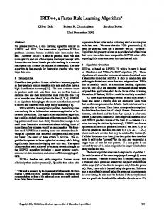
Fig. 1 Errors of the predictions made by WHAT with four different sampling policies. Note that, on the y-axis, lower errors are better.

– The ×—× lines in Figure 1 show a baseline result where data from the performance scores of 100 % of configurations were used by CART to build a runtime predictor.


13

– The other lines show the results using the sampling methods defined in Section 3.2. Note that these sampling methods used runtime data only from a subset of 100 % of the performance scores seen in configurations from 0 to X %. In Figure 1, lower y-axis values are better since this means lower prediction errors. Overall, we find that: – Some of the subject systems exhibit large variances in their error rate, below X = 40 % (e.g., BDBC and BDBJ). – Above X = 40 %, there is little effect on the overall change of the sampling methods. – Mostly, S3 shows the highest overall error, so that it cannot be recommended. – Always, the ×—× baseline shows the lowest errors, which is to be expected since predictors built on the baseline have access to all data. – We see a trend that the error of S1 and S2 are within 5 % of the baseline results. Hence, we can recommend these two minimal sampling methods. Figure 2 provides information about which of S1 or S2 we should recommend. This figure displays data taken from the X = 40 % point of Figure 1 and displays how many performance scores of configurations are needed by our sampling methods (while reflecting on the configurations seen in the range 0 ≤ X ≤ 40). Note that: – S3 needs up to thousands of performance scores points, so it cannot be recommended as minimal-sampling policy; – S2 needs twice as much performance scores as S1 (S2 uses two samples per leaf cluster while S1 uses only one). – S1 needs performance scores only for a few dozen (or less) configurations to generate the predictions with the lower errors seen in Figure 1. Combining the results of Figure 1 and Figure 2, we conclude that: S1 is our preferred spectral sampling method. Furthermore, the answer to RQ1 is “yes”, because applying WHAT, we can (a) generate runtime predictors using just a few dozens of sample performance scores; and (b) these predictions have error rates within 5 % of the error rates seen if predictors are built from information about all performance scores.

5.2 RQ2 Do less data used in building prediction models cause larger variances in the predicted values? Two competing effects can cause increased or decreased variances in performance predictions. In our study, we report standard deviation (σ ) as a measure of variances in the performance predicitons. The less we sample the configuration space, the less we constrain model generation in that space. Hence, one effect that can be expected is that models learned from too few samples exhibit large variances. But, a compensating effect can be introduced by sampling from the spectral space since that space contains fewer confusing or correlated variables than the raw configuration space.

14

Vivek Nair et al.

Fig. 2 Comparing evaluations of different sampling policies. We see that the number of configurations evaluated for S2 is twice as high as S1 , as it selects 2 points from each cluster, where as S1 selects only 1 point.

Figure 3 reports which one of these two competing effects are dominant. Figure 3 shows that after some initial fluctuations, after seeing X = 40 % of the configurations, the variances in prediction errors reduces to nearly zero, which is similar to the results in figure 1. Based of the results of Figure 3, we answer RQ2 with “no”: Selecting a small number of samples does not necessarily increase variance (at least to say, not in this domain).

5.3 RQ3 Can “good” surrogate models (to be used in optimizers) be built from minimal samples?


15

Fig. 3 Standard deviations seen at various points of Figure 1.

The results of answering RQ1 and RQ2 suggest to use WHAT (with S1 ) to build runtime predictors from a small sample of data. RQ3 asks if that predictor can be used by an optimizer to infer what other configurations correspond to system configurations with fast performance scores. To answer this question, we ran a random set of 100 configurations, 20 times, and related that baseline to three optimizers (GALE [21], DE [36] and NSGA-II [6]) using their default parameters.

16

Vivek Nair et al.

When these three optimizers mutated existing configurations to suggest new ones, these mutations were checked for validity. Any mutants that violated the system’s constraints (e.g., a feature excluding another feature) were rejected and the survivors were “evaluated” by asking the CART surrogate model. These evaluations either rejected the mutant or used it in generation i + 1, as the basis for a search for more, possibly better mutants. Figure 4 shows the configurations found by the three optimizers projected onto the ground truth of the performance scores of nearly all configurations (see Section 4.2). Again note that, while we use that ground truth for the validation of these results, our optimizers used only a small part of that ground-truth data in their search for the fastest configurations (see the WHAT + S1 results of Figure 2). The important information of Figure 4 is that all the optimized configurations fall within 1 % of the fastest configuration according to the ground truth (see all the lefthand-side dots on each plot). Table 2 compares the performance of the optimizers used in this study. Note that the performances are nearly identical, which leads to the following conclusions: Based on the results of figure 4 answer to RQ3 is “yes”: For optimizing performance scores, we can use surrogates built from few runtime samples. The choice of the optimizer does not critically effect this conclusion.

Table 2 The table shows how the minimum performance scores as found by the learners GALE, NSGA-II, and DE, vary over 20 repeated runs. Mean values are denoted µ and IQR denotes the 25th–75th percentile. A low IQR suggests that the surrogate model build by WHAT is stable and can be utilized by off the shelf optimizers to find performance-optimal configurations. Searcher GALE

Apache BDBC BDBJ LLVM SQLite X264

DE

NSGAII

Mean

IQR

Mean

IQR

Mean

IQR

870 0.363 3139 202 13.1 248

0 0.004 70 3.98 0.241 3.3

840 0.359 3139 200 13.1 244

0 0.002 70 0 0 0.003

840 0.354 3139 200 13.1 244

0 0.005 70 0 0.406 0.05

5.4 RQ4 How good is WHAT compared to the state of the art of learning performance predictors from configurable software systems? We compare WHAT with the three state-of-the-art predictors proposed in the literature [35], [15], [29], as discussed in Section 2. Note that all approaches use


17

Fig. 4 Solutions found by GALE, NSGA-II, and DE (shown as points) laid against the ground truth (all known configuration performance scores). It can be observed that all the optimizers can find the configuration with lower performance scores.

regression-trees as predictors, except Siegmund’s approach, which uses a regression function derived using linear programming. The results were studied using nonparametric tests, which was also used by Arcuri and Briand at ICSE ’11 [25]). For testing statistical significance, we used non-parametric bootstrap test 95% confidence [9] followed by an A12 test to check that any observed differences were not

18 Rank Apache 1 1 1 1 1 BDBC 1 2 2 2 3 BDBJ 1 1 1 2 2 LLVM 1 1 1 1 2 SQLite 1 2 3 3 4 x264 1 1 1 1 2

Vivek Nair et al. Approach

Mean MRE(µ)

STDev(σ )

Sarkar Guo(PW) Siegmund WHAT Guo(2N)

7.49 10.51 10.34 10.95 13.03

0.82 6.85 11.68 2.74 15.28

Sarkar Siegmund WHAT Guo(PW) Guo(2N)

1.24 6.14 6.57 10.16 49.90

1.46 4.41 7.40 10.6 52.25

Guo(2N) Guo(PW) WHAT Sarkar Siegmund

2.29 2.86 4.75 5.67 6.98

3.26 2.72 4.46 6.97 7.13

Guo(PW) WHAT Sarkar Guo(2N) Siegmund

3.09 3.32 3.72 4.99 8.50

2.98 1.05 0.45 5.05 8.28

Sarkar WHAT Guo(2N) Guo(PW) Siegmund

3.44 5.60 8.57 8.94 12.83

0.10 0.57 7.30 6.24 17.0

Sarkar WHAT Guo(2N) Guo(PW) Siegmund

6.64 6.93 7.18 7.72 31.87

1.04 1.67 7.07 2.33 21.24

#Evaluations

s

s

s s s

s

s s s s

s

s

s

s s s

s

55 29 29 16 18

s

s s s s

s

s

s s

191 139 64 139 36

s

52 48 16 48 57

s

64 32 62 22 43 925 64 78 566 566

s

s

93 32 32 81 81

Fig. 5 Mean MRE(µ) seen in 20 repeats. Mean MRE is the prediction error as described in Equation 3 and STDev (σ ) is the standard deviation of the MREs found during multiple repeats. Lines with a a dot in the s ) show the mean as a round dot withing the IQR (and if the IQR is very small, only middle (e.g. a round dot will be visible). All the results are sorted by the mean values: a lower mean value of MRE is better than large mean value. The left-hand side column (rank) ranks the various techniques for e.g. when comparing various techniques for Apache, all the techniques have the same rank since their mean values are not statistically different. Rank is computer using Scott-Knott, bootstrap 95% confidence, and the A12 test.

trivially small effects; i.e. given two lists X and Y , count how often there are larger numbers in the former list (and there there are ties, add a half mark): a = ∀x ∈ X, y ∈ Y #(x>y)+0.5∗#(x=y) (as per Vargha [38], we say that a “small” effect has a < 0.6). |X|∗|Y | Lastly, to generate succinct reports, we use the Scott-Knott test to recursively divide our optimizers. This recursion used A12 and bootstrapping to group together subsets that are (a) not significantly different and are (b) not just a small effect different to


19

each other. This use of Scott-Knott is endorsed by Mittas and Angelis [25] and by Hassan et al. [13]. As seen in Figure 5, the FW heuristic of Siegmund et al. (i.e., the sampling approach using the fewest number of configurations) has the higher errors rate and the highest standard deviation on that error rate (four out of six times). Hence, we cannot recommend this method or, if one wishes to use this method, we recommend using the other sampling heuristics (e.g., HO, HS) to make more accurate predictions (but at the cost of much more measurements). Moreover, the size of the standard deviation of this method causes further difficulties in estimating which configurations are those exhibiting a large prediction error. As to the approach of Guo et al (with PW), it does not standout on any of our measurements. Its error results are within 1% of WHAT; its standard deviations are usually larger and it requires much more data than WHAT (Evaluations column of the figure 5). In terms of the number of measure samples required to build a model, the righthand column of Figure 5 shows that WHAT requires the fewest samples except for two cases: the approach of Guo et al. (with 2N) working on BDBC and LLVM. In both these cases, the mean error and standard deviation on the error estimate is larger than WHAT. Furthermore, in the case of BDBC, the error values are µ = 14 %, σ = 13 %, which are much larger than WHAT’s error scores of µ = 6 %, σ = 5 %. Although the approach of Sarkar et al. produces an error rate that is sometimes less than the one of WHAT, it requires the highest number of measurements. Moreover, WHAT 's accuracy is close to Sarkar's approach (1% to 2%) difference). Hence, we cannot recommend this approach, too. Table 3 shows the number of evaluations used by each approaches. We see that most state-of-the-art approaches often require many more samples than WHAT. Using those fewest numbers of samples, WHAT has within 1% to 2 % of the lowest standard deviation rates and within 1 to 2 % of lowest error rates. The exception is Sarkar’s approach, which has 5 % lower mean error rates (in BDBC, see the Mean MRE column of figure 5). However, as shown in right-hand side of Table 3, Sarkar’s approach needs nearly three times more measurements than WHAT. To summarize, there are two cases in Figure 5 where WHAT performs worse than, at least, one other method: – SQLite: The technique proposed by Sarkar et al. does better than WHAT (3.44 vs 5.6) but, as shown in the final column of Figure 5, does so at the cost of 925 64 ≈ 15 times more evaluations that WHAT. In this case, a pragmatic engineer could well prefer our solution over that of Sarkar et al. (since number of evaluations performed by Sarkar et al.more than an order of magnitude than WHAT). – BDBC: Here again, WHAT is not doing the best but, compared to the number of evaluations required by all other solutions, it is not doing particularly bad. Given the overall reduction of the error is small (5 % difference between Sarkar and WHAT in mean error), the cost of tripling the data-collection cost is often not feasible in a practical context and might not justify the small additional benefit in accuracy.

20

Vivek Nair et al.

Table 3 Comparison of the number of the samples required with the state of the art. The grey colored cells indicate the approach that requires the lowest number of samples. We notice that WHAT and Guo (2N) uses less data compared to the other approaches. The high fault rate of Guo (2N) accompanied with high variability in the predictions makes WHAT our preferred method. Samples

Apache BDBC BDBJ LLVM SQLite X264

Siegmund

Guo (2N)

Guo (PW)

Sarkar

WHAT

29 139 48 62 566 81

181 36 52 22 78 32

29 139 48 64 566 81

55 191 57 43 925 93

16 64 16 32 64 32

Based on the results of figure 5, we answer RQ4 with “yes”, since WHAT yields predictions that are similar to or more accurate than prior work, while requiring fewer samples.

6 Why does it work? In this section, we present an in-depth analysis to understand why our sampling technique (based on a spectral learner) achieves such low mean fault rates while being stable (low variance). We hypothesize that the configuration space of the system configuration lie on a low dimensional manifold.

6.1 History Menzies et. al [24] demonstrated how to exploit the underlying dimension to cluster data to find local homogeneous data regions in an otherwise heterogeneous data space. The authors used an algorithm called WHERE (see section 3.3), which recurses on two dimensions synthesized in linear time using a technique called FASTMAP [11]. The use of underlying dimension has been endorsed by various other researchers [1, 2, 7, 41]. There are numerous other methods in the literature, which are used to learn the underlying dimensionality of the data set such as Principal Component Analysis (PCA) [19] 8 , Spectral Learning [32] and Random Projection [3]. These algorithms use different techniques to identify the underlying, independent/orthogonal dimensions to cluster the data points and differ with respect to the computational complexity and accuracy. We use WHERE since it computationally efficient O(2N), while still being accurate. 8

WHERE is an approximation of the first principal component


21

6.2 Testing Technique Given our hypothesis the configuration space lies in a lower dimensional hyperplane — it is imperative to demonstrate that the intrinsic dimensionality of the configuration space is less than the actual dimension. To formalize this notion, we borrow the concept of correlation dimension from the domain of physics [14]. The correlation dimension of a dataset with k items is found by computing the number of items found at distance withing radius r (where r is the Euclidean distance between two configurations) while varying r. This is then normalized by the number of connections between k items to find the expected number of neighbors at distance r. This can be written as: n n 2 (4) C(r) = ∑ ∑ I(||xi , x j || < r) k(k − 1) i=1 j=i+1 ( 1, if x