Faster Reinforcement Learning After Pretraining Deep Networks to Predict State Dynamics Charles W. Anderson∗ , Minwoo Lee† and Daniel L. Elliott‡ Department of Computer Science Colorado State University Fort Collins, Colorado 80523-1873 Email: ∗
[email protected], †
[email protected], ‡
[email protected] Abstract—Deep learning algorithms have recently appeared that pretrain hidden layers of neural networks in unsupervised ways, leading to state-of-the-art performance on large classification problems. These methods can also pretrain networks used for reinforcement learning. However, this ignores the additional information that exists in a reinforcement learning paradigm via the ongoing sequence of state, action, new state tuples. This paper demonstrates that learning a predictive model of state dynamics can result in a pretrained hidden layer structure that reduces the time needed to solve reinforcement learning problems.
I.
I NTRODUCTION
Multilayered artificial neural networks are receiving much attention lately as key components in the newly-labeled field of “deep learning” research. When applied to large data sets, such as images, videos, and speech, straightforward algorithms for training deep networks often result in state-of-the-art classification performance. As pointed out by Mnih, et al. [1], [2], reinforcement learning differs from the supervised learning methods commonly used to fine-time deep networks. Reinforcement learning problems require learning from evaluations of a learning agent’s behavior, or reinforcements, rather than from correct, known outputs from a training set of data. Mnih, et al., go on to identify key issues that must be addressed to develop deep learning approaches to reinforcement learning (RL). These issues stem from the fact that as an RL agent learns, its behavior changes which forces the world in which the RL agent is performing to enter new states. The interactions between the RL agent and its world result in an evolving set of novel experiences, a situation much different from the supervised learning framework with a fixed set of training data. Other issues are due to reinforcement value often being delayed and sparse in time. All of these issues result in the perception that algorithms for solving RL problems are inefficient, requiring a large number of interactions to find approximately optimal policies—functions that map sensed world states into actions. A common approach to solving RL problems involves the learning of a value function that predicts the expected sum of future reinforcements from sensed world states and actions taken. Numerous lines of research have been directed at decreasing the number of interactions required to solve RL problems. Best results for many RL problems can only be achieved if the value function is designed for continuouslyvalued states and actions, for which convergence proofs have just begun to appear in the literature [3], [4]. On the practical
side, current algorithms for solving RL problems using continuous function approximators are still very slow, requiring a large number of samples of states and actions to learn successful policies. An obvious way to reduce the number of samples needed is to use a model of the world to generate additional samples that approximate those that could be obtained from the real world. This is the approach taken by Sutton in his DYNA algorithm [5]. Models may also be used to evaluate multiple future action sequences by applying them to the model, as in Deisenroth and Rasmussen’s PILCO algorithm [6]. Another use of a learned model is introduced with the approach described here. It can easily be combined with the model-based approaches just mentioned, but we do not do so here. Instead, our focus is on transferring the state-action representation that develops from learning the model to the process of learning the Q function to predict reinforcements. The model’s representation is used to initialize the Q function’s representation, the hypothesis being that the model’s representation contains features similar to those required to predict reinforcements. To the extent that this is true for a given RL problem, a reduction in the number of required samples will be obtained. This transfer of representation can also be thought of as a way to pretrain the Q function using states observed from actions applied using any policy, even a random one. This pretraining takes place before any information related to the RL problems goals are presented, i.e., the reinforcement signals. It is well accepted that prediction allows animals to anticipate advantageous and disastrous outcomes of their actions. Such prediction is well-studied in the animal learning literature as characterized by instrumental and classical conditioning paradigms, upon which the reinforcement learning field is based. Here we investigate a more subtle utility of a predictive model—a detailed representation of the world that provides a framework for estimating future reinforcements. In this paper, neural networks are used as Q function approximators, or Q networks. The hidden layers of the neural networks comprise the representation that is transferred from the state dynamics prediction problem to the reinforcement learning problem. In Section II, neural networks as approximations of the Q function are reviewed. Recent contributions in deep learning for reinforcement learning are also summarized. In Section III our approach to pretraining the Q network is described. Experiments and results of this approach applied to
several dynamic control tasks are summarized in Section IV. II.
Q N ETWORKS
Neural networks have been used as continuous Q function approximators since the 1980’s [7], [8], [9], [10]. These works and many that followed use stochastic gradient descent to optimize the Q network’s approximation to the expected sum of future reinforcements, and so were rather inefficient in terms of the number of samples needed. More efficient methods for training neural networks in supervised learning problems developed around approximations to second-order gradients. One way to take advantage of such methods in the RL framework is to combine sequences of samples into batches from which second order and conjugate gradient information can be obtained. An example is the Neural Fitted-Q approach of Riedmiller [11]. Lange and Riedmiller [12] combined this approach with new ideas from the deep learning community for pretraining the hidden layers of a neural network. The hidden layers of a neural network were trained to form auto-encoders first. Then these layers were used as the initialization of a Q network. Lange and Riedmiller’s approach, and the approach presented in this paper, demonstrate that for multilayered neural networks, transferring the representation can be as simple as replacing the output layer. Lange and Riedmiller’s optimize the reproduction of the input by forcing information flow through hidden layers of fewer units than input components, a form of nonlinear dimensionality reduction akin to the early work of Kramer [13]. The resulting lower dimensional representation is likely to reduce the number of samples required to solve a subsequent RL problem. Without such pretraining, the lower dimensional representation would have to be learned while the RL problem is being solved, requiring many more samples. Our approach will also develop a nonlinear dimensionality reduction if the network structure includes hidden layers of fewer units than input dimensions. However, there is a fundamental difference between Lange and Riedmiller’s approach and our approach in the optimization being performed during pretraining. Instead of reconstructing the input in auto-encoder fashion, our approach is to model the dynamics of the world and the effects on it of the agent’s actions. It is expected that features that capture aspects of the world’s dynamics will be very useful for predicting future reinforcement, leading to a reduction in required samples beyond that obtained with autoencoder pretraining. III.
P RETRAINING OF H IDDEN U NITS
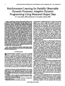
The neural network structure used here is shown in Figure 1. The hidden units of the neural network form adaptive representations which the output units combine to approximate the desired function. The figure shows the usual Q function output, but it also shows additional outputs representing changes in state 𝑠. A single neural network can be trained to predict state changes and to predict the sum of future reinforcements, i.e., the Q function, as shown in Figure 1. Details of the computations implicit in this figure are presented later. The hypothesis explored in this paper is that a representation in the hidden units that is useful in predicting state changes will also be helpful in predicting the sum of future reinforcements. The
Fig. 1.
Neural network for learning state prediction and Q function
usual practice of using neural networks to learn Q functions is to provide just the single Q output. For cases when non-zero reinforcements are rare, as is the case in many episodic tasks, like games, the error feedback from state change prediction will add a tremendous amount of guidance in learning a good representation. “State” and 𝑠𝑡 are used here to refer to all observable measurements of the system with which a reinforcement learning agent interacts. It is not meant that the complete state of the system is being observed. In practice it is usually impossible to fully measure the state of the RL agent’s world. “State” will continue to be used to refer to observables in this paper. Also, unobservable state means the dynamics of the observed variables are stochastic in nature. The algorithms used here for modeling of state dynamics and of future reinforcements minimize expected values and can therefore deal with some degree of randomness in observable variables and reinforcement. To pretrain the neural network, samples of state, 𝑠𝑡 , action, 𝑎𝑡 , and next state, 𝑠𝑡+1 are collected. Each sample of 𝑠𝑡 and 𝑎𝑡 form an input vector to the network. The correct output, or target value, for this input vector is 𝑠𝑡+1 − 𝑠𝑡 . Just the next state, 𝑠𝑡+1 , could also be used as the target value, but state from one time step to the next are often very similar, so the neural network is driven to learn an identity map and more training is required to learn the small variations needed to accurately predict next state. The input and target output values are combined into matrices and Møller’s Scaled Conjugate Gradient (SCG) algorithm [14] is used to minimize the mean squared error in the output of the neural network. SCG is a conjugate gradient method that replaces the typical line-search step by an approximate second-order minimization. During this pretraining stage, no knowledge is used of the objective of the reinforcement learning problem, and the Q value output of the neural network is ignored. After pretraining, steps similar to Riedmiller’s NeuralFitted Q algorithm are taken. Minibatches of 𝑠𝑡 , 𝑎𝑡 , reinforcement, 𝑟𝑡+1 , 𝑠𝑡+1 , and 𝑎𝑡+1 are collected. Actions 𝑎 are selected using the 𝜖-greedy algorithm. Møller’s SCG algorithm is again applied to train the output Q value to approximate the sum of future reinforcement. During this phase the state change outputs are ignored. The SARSA algorithm [15] is followed to form the error being minimized as summarized below. The Q output value, 𝑄(𝑠𝑡 , 𝑎𝑡 ), that is output by the network is determined by inputs 𝑠𝑡 and 𝑎𝑡 . We wish this function to
form the approximation 𝑄(𝑠𝑡 , 𝑎𝑡 ) ≈ 𝐸[
∞ ∑
𝛾 𝑘 𝑟𝑡+𝑘+1 ],
𝑘=0
where 0 < 𝛾 ≤ 1 is the discount factor. Actions are chosen using an 𝜖-greedy policy 𝜋(𝑠𝑡 ), { argmax 𝑄(𝑠𝑡 , 𝑎) with probability 1 − 𝜖, 𝑎∈𝐴 𝜋(𝑠𝑡 ) = 𝑧 ∼ 𝒰 (𝐴) with probability 𝜖, where 𝑧 is a uniformly-distributed random variable drawn from the set of valid actions 𝐴. If each minibatch consists of 𝑛 samples collected from time 𝑡1 through time 𝑡𝑛 , then the SARSA error to be minimized for each minibatch is 𝑡𝑛 ∑
(𝑟𝑡+1 + 𝛾𝑄(𝑠𝑡+1 , 𝑎𝑡+1 ) − 𝑄(𝑠𝑡 , 𝑎𝑡 ))2
𝑡=𝑡1
The gradient of this error for a minibatch of 𝑛 samples, (𝑠𝑡 , 𝑎𝑡 , 𝑟𝑡+1 , 𝑠𝑡+1 , 𝑎𝑡+1 ) for 𝑡 = 𝑡1 , . . . , 𝑡𝑛 , with respect to the weights of the neural network drives the error minimization performed by Møller’s SCG algorithm. It is important to not overfit the 𝑄 function to each minibatch of samples. Each minibatch is a sample that is limited to the particular sequence of world states experienced. Therefore, the SCG algorithm is applied for a small number of iterations for each minibatch. For the experiments reported here, it is applied for 20 iterations only. Experience-replay was found to reduce the total number of samples for the reported experiments. This was performed by calculating new 𝑄 values for the minibatch samples and retraining with SCG for another 20 iterations. Experience-replay was repeated 10 times for each minibatch. In the following section, results are summarized for experiments on two RL problems involving the control of simulated dynamic systems. Performance is compared for different numbers of pretraining samples, including zero. IV.
E XPERIMENTS
Two simple dynamic systems were used to investigate the advantage of pretraining. The first system is a simple mass, or cart, on a one-dimensional track. The second is a benchmark cart and pole system for which the pole is to be balanced. We used a unique simulation that includes cart collisions with the ends of the track. A. Cart Consider a mass, or cart, that can be pushed left or right as it moves along a horizontal track with walls at positions 1 and 10 and that has a region of increased friction from position 2 to 4, illustrated in Figure 2. A reinforcement learning problem is defined by requiring a sequence of pushes that cause the cart to remain close to a given position. Let the state of the cart at time 𝑡 be 𝑠𝑡 = (𝑥𝑡 , 𝑥˙ 𝑡 )𝑇 and the push at time 𝑡 be 𝑎𝑡 ∈ {−1, 0, 1}, which will be referred to as the action. The evolution of the state can be simulated using Euler’s method by
Fig. 2. Dynamic cart on a one-dimensional track with increased friction from position 2 to 4.
[
] [ ] [ ] 𝑥𝑡+1 𝑥𝑡 𝑥˙ 𝑡 = +Δ 𝑥˙ 𝑡+1 𝑥˙ 𝑡 2𝑎𝑡 − 𝜇𝑡 𝑥˙ 𝑡
where Δ = 0.1, and 𝜇𝑡 is the coefficient of friction given by { 1.0 if 2 < 𝑥𝑡 < 4, 𝜇𝑡 = 0.2 otherwise. Inelastic collisions with walls is simulated by bounding 𝑥 by 1 and 10 and setting 𝑥˙ = 0. Let 𝑔𝑡 be the goal position, from 1 to 10. The reinforcement value at time 𝑡 is { 1 if ∣𝑥𝑡 − 𝑔𝑡 ∣ < 2, 𝑟𝑡 = 0 otherwise. To make this task more challenging, five additional state variables are used that are simply drawn from a uniform distribution from 0 to 1. During pretraining, changes in these variables are included in optimizing the state-change model. Other ways of making this simple task more challenging are to add hills to the track and to change the effect of actions in certain states [16]. The structure of the Q network for this experiment is eight inputs, 20 hidden units in a single hidden layer, and eight outputs, or 8-20-8. The eight inputs include the two state variables, position and velocity, the five random-variables, and the action. The eight outputs are predicted changes in the two state variables, predicted changes in the five random variables, and the 𝑄 value. All units also receive a constant 1 bias input. The hidden units use the symmetric tanh activation function and the output units are linear. Since the SCG algorithm determines step size, learning rates are not needed. To generate samples for pretraining, the cart is initialized to a random position with zero velocity and a random goal position. Actions are selected randomly. Every 100 samples the goal is changed to a new random value. During pretraining, the Q output value is ignored. After pretraining, the state change outputs are ignored and training of the Q output is performed. Again, the cart is initialized to a random position with zero velocity and a random goal position. An action is chosen with the 𝜖-greedy algorithm and applied to the cart and the next state and reinforcement is observed. This is repeated for 1000 steps, with the goal changing to a new random value every 100 steps. The minibatch of 1000 steps is used to update the Q network while ignoring the state change outputs. This is repeated for 100 such minibatches. The value of 𝜖 is set to the constant 0.1 while training and the value of 𝛾 is set to 0.9. To evaluate the effect of pretraining the neural network to minimize predicted state changes, the above procedure was run for different numbers of pretraining samples. This was repeated 30 times for each number of pretraining samples. During each run, performance is measured by the mean of all
0.6
Mean of R Over All Batches
0.4
0.5
Fig. 5.
Cart-Pole Swing Up Task.
B. Cart-Pole Swing Up
0.2
0.3
Mean of Reinforcement
0.7
Mean of R Last 10% of Batches
0
1000
2000
3000
4000
Number of Samples for State Change Prediction
Fig. 3. Advantage of pretraining to predict state change, shown by mean of reinforcement achieved for an increasing number of pretrained samples. The mean of reinforcement over all training samples and over the samples in the final 10 minibatches are shown.
Adding a pole to the cart that swings in two dimensions results in the benchmark pole-balancing problem, first studied in the reinforcement learning field by Barto, et al. [17]. This benchmark problem is modified here in two ways. First, the dynamic system is simulated using pybox2d, a python package based on the box2d library. This allows realistic collisions with the ends of the track. The second difference is that the pole can swing through the full 360 ∘ rather than being restricted to a small angle near the upright position that was used in the original benchmark problem. Other published results for pole-balancing problems allow the full angle range, but many incorporate a model of the dynamics that is not used here. Figure 5 shows the cart and pole on the track.
−3
−1
0
x⋅
1
2
3
4
The state of this system is four-dimensional: the cart position, 𝑥𝑡 , its velocity, 𝑥˙ 𝑡 , the pole angle, 𝜃𝑡 , and its angular velocity, 𝜃˙𝑡 . When the pole is straight up, 𝜃𝑡 = 0 ∘ , and when it swings down it approaches negative or positive 180 ∘ . The reinforcement function for this problem is defined in terms of the angle: ⎧ if ∣𝜃𝑡 ∣ < 45 ∘ , ⎨1 𝑟𝑡 = −1 if ∣𝜃𝑡 ∣ > 135 ∘ , ⎩ 0 otherwise. 0
2
4
6
8
10
x
Fig. 4. Successful control by trained neural network shown by state evolution from multiple initial values, marked by filled circles. The goal is at position 8.
reinforcements and the mean of the reinforcements received during the last 10 minibatches. Figure 3 shows the two performance measures versus the number of pretraining samples. Recall that reinforcement is zero until within 2 of the goal, at which time the reinforcement is 1. So, a mean of 0.7 means the goal region is reached quickly. This figure shows that with no pretraining, the goal is rarely reached. Performance steadily improves with more pretraining samples, with the most rapid rise being from 0 to 1000 pretraining samples. The similarity in the mean of all reinforcements and of the last 10% shows that good performance is achieved early in each run. Good performance is confirmed by starting the system in multiple initial states and observing the evolution of the state under the control of the trained neural network using the 𝜖-greedy policy with 𝜖 = 0. This is shown in Figure 4 with the goal set at position 8.
The dynamics of the system are simulated at a sampling rate of 30 Hz and a new action is applied by the RL agent at a 15 Hz rate. For this experiment, the Q network has five inputs, one to five hidden layers of 20 units each, and five outputs. The inputs are the four state variables and the action. The outputs are predictions of the changes in the four state variables and the 𝑄 value. To collect pretraining samples, the cart-pole system was started in the center of the track with the pole hanging down. Random actions were applied and resulting states collected. The SCG algorithm was run for 1000 iterations to minimize the squared error in the predicted state change, while ignoring the output 𝑄 value. After pretraining, the cart-pole was again started in the center with the pole hanging down. The 𝜖-greedy policy was used to choose actions, with 𝜖 constant at a value of 0.1. 100 minibatches of 1000 samples were collected, with SCG applied for each minibatch for 20 iterations, repeated for 10 repetitions of experience-replay, all while ignoring the state change output values. The value of 𝛾 was 0.9. At the conclusion of training the Q network for 100 minibatches, a final testing stage was conducted. The cart-pole was initialized to fifteen different starting states, at three different
Fig. 6. Mean reinforcement value received during the testing phase for Q networks pretrained with different numbers of pretraining samples.
positions along the track, from -2 to 2 meters, and five different angles, from −180 ∘ to 180 ∘ , and the Q network was allowed to control the system using 𝜖 = 0 for 2000 steps. The mean of the reinforcement values over these 15 × 2000 = 30000 steps, or about 33.3 simulated minutes, was calculated to test the final performance of the trained Q network. For each network size and number of pretraining steps, the experiment was repeated 100 times. Results shown in Figure 6 are the means of reinforcement received during testing averaged over these 100 runs, with 90% confidence intervals. During the final evaluation the pole is initialized at zero degrees, pointing up, for only three of the fifteen initial states, so a mean reinforcement of 1 cannot be obtained. The best result is about 0.6 for the 5-20-20-20-5 network pretrained with 2000 samples, equivalent to about 2.2 simulated minutes. The largest improvement is seen in comparing no pretraining (0 samples) with pretraining of 1000 samples. For networks with two or three hidden layers the improvement due to pretraining was from a mean reinforcement of about 0.4 to 0.6. For networks with four or five hidden layers the improvement was from about 0.2 to 0.4 mean reinforcement. The difference in performance with pretraining for the smallest network, 520-5, is not clear. The 5-20-5 network can achieve better performance with additional training. Note that even for the largest network, 5-20-20-20-2020-5, the typical deep-learning approach of pretraining the initial hidden layer in an unsupervised way is not followed here. The SCG algorithm appears to be sufficiently efficient at propagating state prediction errors and Q value errors to early layers that this kind of pretraining was not needed. Figure 7 shows the behavior of the cart-pole system and the greedy actions selected during one of the test phases for a 520-20-5 network pretrained with 1000 samples. In this phase, the cart is started near the left side and the pole is started in the up position (0 ∘ ). Actions are selected that push the cart towards the center of the track and, after several swings of the
Fig. 7. One of the test runs, started at 𝑥 = −2 and 𝜃 = 0, with 𝜖 = 0. The positive action, a push to the right (fourth graph) is first applied, which directs cart towards center of track (first graph), but pushes the pole to swing through the bottom (second graph). Then, actions are chosen that swing the pole back and forth through the bottom five times until it is successfully swung up to 0 degrees where it remains balanced for the remainder of the test session. The cart is brought back to the center of the track where it remains. Reinforcement values received (fourth graph) are negative when the pole swings through the bottom and positive when the pole is near the top.
pole through the bottom, the pole is swung up to its balanced position where it remains. Figure 8 shows the reinforcement values received by a 520-20-20-5 Q network during training, averaged over minibatches of 1000 samples and averaged over 50 runs. With pretraining of 2000 samples, the final mean reinforcement value is almost 0.6, while without pretraining it reaches about 0.3. When reinforcement surpasses zero the pole is near the balancing position more often than it is near the bottom position. With pretraining this occurs after about 24.4 simulated minutes (24.4 ≈ 22 minibatches ×1000 samples/minibatch ÷ 15 samples/second ÷ 60 seconds/minute). Without pretraining zero reinforcement is not surpassed until about 67 simulated minutes (67 ≈ 60 minibatches × 1000 samples/minibatch ÷ 15 samples/second ÷ 60 seconds/minute). V.
D ISCUSSION
In a realistic setting, one should consider the additional samples required for pretraining in the total training time. The following simple experiment examines this for a simple Markov Decision Problem (MDP) with two states, State 0 and State 1, and two actions, Action 0 and Action 1. Action 1 results in a change in state and Action 0 does not. Therefore, the next state function is the exclusive-or function of the state and action inputs. The exclusive-or was one of the early functions used to test learning in two-layer neural networks. The reinforcements for this MDP are 1 for being in State 1
Reinforcement Received (0 to 1)
mean r final r
Fraction of Samples Used for Pre-Training Fig. 9. Exclusive-or MDP: Best performance is achieved when only 0.7 of the samples are used for Q learning and the remaining 0.3 samples are used for pretraining. Fig. 8. Mean reinforcement value during Q training for the cart-pole swing up task, with and without pretraining.
and 0 for being in State 0. The total number of samples of states, actions and reinforcements was fixed. Only the fraction of them used for pretraining was varied; using 0.2 of the samples for pretraining left only 0.8 of the samples for doing reinforcement learning to solve the reinforcement optimization problem. Figure 9 shows the results as the mean reinforcement received during training and the mean reinforcement received in the last few trials is plotted. The experiment was repeated 100 times. At the left end of the graph, for 0 samples used for pretraining, all samples were used for reinforcement learning and achieved an average reinforcement of about 0.5. Recall that the reinforcement values were 0 and 1, so the maximum value is 1. Performance peaks at about 0.3 of the samples used for pretraining and 0.7 used for reinforcement learning. Performance then decreases as more of the samples are used for pretraining and fewer for reinforcement learning. This result shows that for this problem, with a fixed number of sample interactions, a neural network RL agent can achieve better performance by using some of the samples for pretraining to predict state dynamics before using the remaining samples to solve the RL problem.
predict the sum of future reinforcements, while ignoring the state change output variables. Experiments with simple dynamic systems, including the swing-up problem for the cart-pole system, show that pretraining in this way does reduce the number of samples required for reinforcement learning. Since the pretraining phase results in a predictive model of the system to be controlled, it would be a simple matter to use it to generate hypothetical samples as in Sutton’s DYNA framework [5]. It is possible that reductions in the number of real samples required resulting from the two uses of the learned model—to generate hypothetical samples and to provide initial hidden layers—will be additive. The advantage afforded by pretraining to predict state change should increase as the complexity of the dynamics and size of the state and action spaces grow. To test this, we are currently testing our approach on the problem of controlling a simulated, multi-segment octopus arm. The difficulty lies in the large number of continuously-valued state and action variables. This is one of the RL benchmark problems [18], but the benchmark problem is a simplified form in which the allowed actions are from a small discrete set. It is hypothesized that with pretraining a practical solution of the full octopus arm problem will be achieved.
The recent success of deep learning in a number of classification problems suggests that deep learning might increase the efficiency of reinforcement learning algorithms. A few publications have appeared showing how pretraining early layers of a neural network in the unsupervised way that is typical in the deep learning community, can lead to benefits for reinforcement learning [1], [2].
A second paradigm to be investigated is the simultaneous learning of predictions of state change and future reinforcement. For tasks in which reinforcement values are rare, many steps occur without any information about how to adjust network weights. However, each step does provide new state information with which adjustments can be made to the network. If common or similar features are found useful for learning state dynamics and Q values, then the advantage of simultaneously learning both will be evident.
This paper demonstrates a different approach to pretraining for reinforcement learning. A neural network is first trained to predict changes in state variables, based on current state and actions. Then the same neural network with pretrained hidden layer weights is further trained to approximate the Q value to
[1] V. Mnih, K. Kavukcuoglu, D. Silver, A. Graves, I. Antonoglou, D. Wierstra, and M. Riedmiller, “Playing atari with deep reinforcement learning,” in NIPS Deep Learning Workshop, 2013.
VI.
C ONCLUSION
R EFERENCES
[2] V. Mnih, K. Kavukcuoglu1, D. Silver, A. Rusu, J. Veness, M. Bellemare, A. Graves, M. Riedmiller, A. Fidjeland, G. Ostrovski, S. Petersen, C. Beattie, A. Sadik, I. Antonoglou, H. King, D. Kumaran, D. Wierstra, S. Legg, and D. Hassabis, “Human-level control through deep reinforcement learning,” Nature, vol. 518, no. 7540, pp. 529–532, February 2015. [3] H. R. Maei, C. Szepesvari, S. Bhatnagar, D. P. adn D. Silver, and R. Sutton, “Convergent temporal-difference learning with arbitrary smooth function approximation,” in Advances in Neural Information Processing Systems, vol. 22. Vancouver, B.C., Canada: MIT Press, December 2009. [4] M. Lee and C. Anderson, “Convergent reinforcement learning control with neural networks and continuous action search,” in Proceedings of IEEE Symposium on Adaptive Dynamic Programming and Reinforcement Learning, Orlando, FL USA, December 2014. [5] R. S. Sutton, “Dyna, an integrated architecture for learning, planning, and reacting,” SIGART Bull., vol. 2, no. 4, pp. 160–163, Jul. 1991. [Online]. Available: http://doi.acm.org/10.1145/122344.122377 [6] M. P. Deisenroth and C. E. Rasmussen, “PILCO: A model-based and data-efficient approach to policy search,” in Proceedings of the International Conference on Machine Learning (ICML 2011), 2011. [7] C. W. Anderson, “Learning and problem solving with multilayered connectionist systems,” Ph.D. dissertation, University of Massachusetts, Amherst, MA, 1986. [8] ——, “Strategy learning with multilayer connectionist representations,” GTE Laboratories, Waltham, MA, Tech. Rep. TR87-509.3, 1987, revision of article that was published in Proceedings of the Fourth International Workshop on Machine Learning, pp. 103–114, June, 1987. [9] ——, “Tower of hanoi with connectionist networks: Learning new features,” in Proceedings of the Sixth International Workshop on Machine Learning, 1989.
[10] G. Tesauro, “Td-gammon, a self-teaching backgammon program, achieves master-level play,” Neural computation, vol. 6, no. 2, pp. 215– 219, 1994. [11] M. Riedmiller, “Neural fitted q iteration—first experiences with a data efficient neural reinforcement learning method,” in Machine Learning: ECML 2005, ser. Lecture Notes in Artificial Intelligence, J. Gama, R. Camacho, P. Brazdil, A. Jorge, and L. Torgo, Eds., no. 3720. Sringer-Verlag, 2005, pp. 317–328. [12] S. Lange and M. Riedmiller, “Deep auto-encoder neural networks in reinforcement learning,” in Proceedings of the International Joint Conference on Neural Networks (IJCNN 2010), Barcelona, Spain, 2010. [13] M. A. Kramer, “Nonlinear principal component analysis using autoassociative neural networks,” AIChE Journal, vol. 37, p. 233243, 1991. [14] M. F. Møller, “A scaled conjugate gradient algorithm for fast supervised learning,” Neural Networks, vol. 6, pp. 525–533, 1993. [15] R. S. Sutton and A. G. Barto, Reinforcement Learning: An Introduction. The MIT Press, 1998. [16] D. Elliott and C. Anderson, “Using supervised training signals of observable state dynamics to speed-up and improve reinforcement learning,” in 2014 IEEE Symposium on Adaptive Dynamic Programming and Reinforcement Learning (ADPRL), Orlando, FL USA, December 2014. [17] A. G. Barto, R. S. Sutton, and C. W. Anderson, “Neuronlike elements that can solve difficult learning control problems,” IEEE Transactions on Systems, Man, and Cybernetics, vol. 13, pp. 835–846, 1983, reprinted in J. A. Anderson and E. Rosenfeld, Neurocomputing: Foundations of Research, MIT Press, Cambridge, MA, 1988. [18] http://www.rl-competition.org/.