uses FLUTE [14] to construct congestion-driven Steiner tree. It then uses pattern routing and multi-source multi- sink maze routing to reduce congestion.
FastRoute 4.0: Global Router with Efficient Via Minimization Yue Xu, Yanheng Zhang and Chris Chu Department of Electrical and Computer Engineering Iowa State university, Ames, IA 50011 Email:{yuexu, yhzhang, cnchu}@iastate.edu
Abstract— The number of vias generated during the global routing stage is a critical factor for the yield of final circuits. However, most global routers only approach the problem by charging a cost for vias in the maze routing cost function. In this paper, we present a global router that addresses the via number optimization problem throughout the entire global routing flow. We introduce the via aware Steiner tree generation, 3-bend routing and layer assignment with careful ordering to reduce via count. We integrate these three techniques into FastRoute 3.0 and achieve significant reduction in both via count and runtime.
I. Introduction As the trend of shrinking feature size and increasing density for VLSI designs continues, there have been many challenges for the development of back-end design tools. They must be able to handle various constraints set by the DFM (Design for Manufacturability) rules. Via is the interconnection between adjacent metal layers. It is a major source for circuit failure. So DFM rules set stringent constraints on vias. Besides, via has large process variation that impacts the timing of circuits. Thus, via minimization has become one of the major targets in backend design. As the last stage of back-end design, routing would determine whether a layout can realize all the interconnections without design rule violation, yet fulfill the timing requirements. So one natural stage to reduce the number of vias is routing. Traditional global routers ignore via count but focus on the oldest yet most important criteria to judge the performance of a global router, the ability to generate solutions without any wire congestion. Kastner et al. [1] proposed a pattern based routing scheme. Hadsell and Madden [2] proposed to guide the routing by amplifying the congestion map with a new congestion cost function. BoxRouter [3] proposed an ILP based approach to simultaneously handle multiple nets and achieved reasonably good routability. FastRoute [4] achieved very fast runtime by exploring congestion-driven RSMT to avoid the extensive usage of maze routing. FastRoute 2.0 [5] im1 This work was partially supported by NSF under grant CCF0540998 and IBM faculty award.
proved the solution quality of FastRoute by introducing monotonic routing and multi-source multi-sink maze routing. In the above mentioned routers, basic pattern routing such as L routing and Z routing generates small number of vias but lacks the effectiveness of solving congestion problem. On the other side, powerful congestion reduction techniques like monotonic routing and maze routing cannot control via generation properly. So even though various methods have been proposed to properly handle congestion, there is little discussion on how to minimize the number of vias. The release of 3D benchmarks in ISPD07 and ISPD08 global routing contests [6][7] requires global routers to consider via count. The earlier consideration of via count in global router will give more flexibility on reducing the via count. Such improvement greatly benefits the quality of solutions. The majority of new routers such as BoxRouter 2.0 [8], Archer [9], NTHU-R [10], MaizeRouter [11] and FastRoute 3.0 [13] employ an efficient scheme of running 2D global routing followed by layer assignment. However, they overly rely on layer assignment to control via count so the 3D solution is restrictive, due to the constraints set by 2D solution. Instead, FGR [12] directly addresses the problem by running 3D maze routing, which can generate better solution at a cost of extremely long runtime. In this paper, we also use the scheme of employing layer assignment after 2D global routing due to its efficiency. However, we propose a global router that addresses the via minimization problem throughout the entire global routing flow. There are three major techniques that significantly reduce the via count: • Via aware Steiner tree generation • 3-bend routing • Layer assignment with careful net and edge ordering The via aware Steiner tree generation produces tree topology that adjusts the number of vias based on congestion and layer information. 3-bend routing is an efficient routing algorithm with detouring option. It has congestion reduction capability like maze routing and effective control on via count like pattern routing. Our layer assignment is a sequential layer assignment algorithm that carefully orders nets and the edges in each net. It then uses efficient dynamic programming to assign layers to each edge.
We integrate the above techniques into FastRoute[4][5][13] and call it FastRoute 4.0. On the benchmarks from 2008 global routing contest held by ISPD, FastRoute 4.0 reduces the number of vias by 13.8% comparing to FastRoute without the three techniques proposed. It can achieve comparable performance as the best global router in the 2008 contest with up to 10 times the speed. The remainder of the paper is organized as follows. In Section II, we overview the framework of FastRoute 4.0. In Section III, we present the three major techniques in detail. We compare the performance with the state of art in Section IV and conclude in Section V.
4.0 first generates the via aware Steiner tree and use pattern routing to initialize a solution. Then we use 3-bend routing and maze routing to solve the congestion problem. When overflow could not be reduced any more, layer assignment finishes the global routing flow.
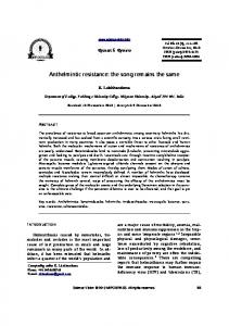
II. Preliminary A. Grid Graph Model FastRoute 4.0 inherit the grid graph model used in FastRoute and extend it into 3D grid graph model, as illustrated in Fig. 1. The boundary on each metal layer between areas above two adjacent global cells is represented by one 3D global grid edge in the perpendicular direction of the original boundary, indicating that wires on the global grid edge are actually crossing the boundary. G
l
o
b
a
l
C
e
l
l
Fig. 2. FastRoute 4.0 Framework
s
III. Via Reduction Techniques A. Via Aware Steiner Tree
G
l
o
b
a
l
E
d
g
e
s
Fig. 1. Global Cells and Corresponding 3D Global Routing Grid Graph
B. Overview of Previous Work and FastRoute 4.0 FastRoute 4.0 is based on the work of FastRoute [4][5][13], which is a powerful and efficient router extremely good at solving congestion problems. FastRoute is a sequential rip-up and reroute tool (RRR) that first uses FLUTE [14] to construct congestion-driven Steiner tree. It then uses pattern routing and multi-source multisink maze routing to reduce congestion. FastRoute 3.0 introduces virtual capacity to adaptively change the capacity associated with each global edge to divert wire usage from highly congested regions to congestion-free regions. As illustrated in Fig. 2, we have integrated the techniques proposed in this paper into FastRoute 3.0, in stages 2, 5, 6 and 8. After the congestion estimation, FastRoute
As most global routers start to consider vias only in the late stages as maze routing and layer assignment, they overly rely on these techniques to solve congestion and reduce via count, where via reduction is often compromised. Moreover, in a common RRR framework, global routers avoid rerouting nets as much as possible to save runtime. So the majority of nets do not go through RRR. These nets keep the original topologies, which are not optimized in terms of via count. Thus, an early consideration of vias in tree topology generation is essential for the quality of global router. Our via aware Steiner tree generation technique further extends congestion driven RSMT proposed in FastRoute[4]. It computes suitable topology at the beginning stage of global routing so that global router will generate less number of via. After analyzing net topologies, we found that different tree topologies have significant impact on via count. As shown in Fig. 3, three topologies are generated for a 7pin net. Assuming horizontal wires are on metal layer 1 and vertical wires on metal layer 2, the three topologies will generate 7, 14 and 9 vias respectively, ignoring the contacts between poly-silicon and metal layers. Here we define two special struectures: Horizontal Tree (H Tree) and Vertical Tree (V Tree). H tree is defined as a rectilin-
ear tree with only one vertical trunks, with all the other trunks in between the vertical trunks and pin nodes to be horizontal. Similarly, vertical tree is defined as a tree with only one horizontal trunk, with all the other trunks in between the horizontal trunk and pin nodes to be vertical. If each net is assigned onto two adjacent metal layers, as our layer assignment algorithm tries to achieve by keeping segments in one net close to each other, H Tree and V Tree are two extremes in terms of the number of vias. Other trees, like the RSMT with smaller wirelength shown in Fig. 3, have via count in between. However, it is not always the case that H Tree would have less number of vias than V Tree. If the resource on metal layer 1 is used up and the net has to go onto layer 2 and 3, it is obvious that V Tree is a better choice. i
V
P
S
H
T
r
e
e
V
T
r
e
e
t
e
i
n
e
i
n
N
o
n
i
m
a
l
d
e
r
T
r
e
Fig. 4. L/Z/U, Monotonic and Maze Routing
a
M
i
congestion problem but cannot control via count effectively. Besides, maze routing and U routing allow detour to strengthen the via reduction capability. Maze routing is most powerful but suffers from long runtime. So the traditional routing techniques all sacrifice one or several quality to improve some others. To address this problem, we propose 3-bend routing, a fast routing technique with enhanced congestion reduction capability than traditional pattern routing and less via than maze routing.
e
Fig. 3. Via Aware Steiner Tree
So we adjust the net topology by the usage and capacity comparisonPbetweenPhorizontal metal layers and P cap cap vertical ones, as P usg(h) / P usg(v) , where cap(h) and (h) (v) P usg(h) is the sum of horizontal capacity and P usage of grid P edges within the bounding box of each net. cap(v) and usg(v) are defined for vertical edges. We multiply this factor with the factor used in FastRoute[4] that generates congested driven RSMT and use the result to scale vertical distances between the pin nodes. Finally, we use the scaled distance in FLUTE to generate adjusted topology for each tree. Trees generated in this way will take consideration of both via count and congestion. For example, if the horizontal resources are more abundant than vertical resources, we scale down the vertical distances. The RSMT computed by FLUTE for such an scaled net will have more horizontal edges. In this way, we manipulate the constitution of horizontal edges and vertical edges in the net structure to reduce via count. The simulation shows a 3% via count reduction after pattern routing stage with less than 1% overhead in wirelength and overflow. B. 3-Bend Routing The most commonly used routing techniques in Global Routing includes L/Z/U routing, monotonic routing and maze routing, as shown in Fig. 4. L/Z/U routing generates limited number of via, has fast speed but is very limited in reducing congestion. Monotonic routing and maze routing, on the contrary, do better job in solving
A 3-bend route is a 2-pin rectilinear connection that has at most three bends and possible detour. It is much more flexible than L/Z/U route on solving congestion problem. Comparing to monotonic route and maze route, 3-bend route has advantage on having less vias. Fig. 5 shows two possible 3-bend routes for a tree edge, S → B → T and S → B ′ → T . No L/Z/U routing can avoid the congested area marked as shades. However, the 3-bend route S → B → T can achieve congestion free routing with least bends possible. (
n
�
1
,
0
)
(
n
�
1
,
m
�
1
)
B
T
B
B
r
e
a
k
’
P
o
i
n
t
S
(
0
,
0
)
(
0
,
m
�
1
)
Fig. 5. 3-Bend Routing
To find the best 3-bend routing path for a 2-pin net, we assume one pin to be the source (S = (ys , xs )) and the other one to be the sink (T = (yt , xt )). Without loss of generality, we assume S is at the lower-left corner and T is at the upper-right corner. We define the possible detouring region as expanding box for each net. It is calculated depending on the size, location and congestion of each net. The larger net with more congestion will have a larger expanding box. The pseudo code to compute the best 3-bend path for an S-T bounding box of size p × q and an expanding box of m × n nodes is given in Fig. 6. In the algorithm, dh (y, x) and dv (y, x) denote the costs for a path going from the point (y, x) horizontally to the left boundary and vertically to the bottom boundary re-
Algorithm 3-Bend Routing 1. 2. 3. 4. 5. 6. 7. 8. 9. 10. 11. 12. 13. 14. 15. 16. 17.
Cbest = +∞ for y = 0 to n − 1 dh (y, 0) = 0 for x = 1 to m − 1 dh (y, x) = dh (y, x − 1) + costh (y, x − 1) for x = 0 to m − 1 dh (0, x) = 0 for y = 1 to n − 1 dv (y, x) = dv (y − 1, x) + costv (y − 1, x) for y = 0 to n − 1 for x = 0 to m − 1 B = (x, y) dL1 (B) = |dh (S)− dh (ys , x)|+ |dv (ys , x)− dv (B)| dL2 (B) = |dh (S)− dh (y, xs )|+ |dv (y, xs )− dv (B)| dL3 (B) = |dh (T ) − dh (yt , x)| + |dv (yt , x) − dv (B)| dL4 (B) = |dh (T )− dh (y, xt )|+ |dv (y, xt )− dv (B)| Compute the cost of four possible 3-bend paths from 4 paths above plus via cost and compare it to Cbest . If better, update best 3-bend path.
Fig. 6. 3-Bend Routing Algorithm
spectively. To balance wirelength and congestion, we use the logistic cost function [4] used in maze routing. Line 2 to Line 9 create two tables that have the cost for a bend-free edge between any points in the bounding box and the left or bottom boundary, from which the cost of a rectilinear path between any two nodes in the bounding box could be easily calculated. A 3-bend path could be concatenated from two L-shaped paths, like using S → B and B → T to form S → B → T . So we add a break point in the expanding box to get all the possible 3-bend paths, calculate their costs and find the best solution. Line 2 to 7 take O(mn) time. Line 8 to 19 also take O(mn) time. So the complexity of 3-bend routing algorithm for a 2-pin net is O(mn), the same as Z routing. It is worth noticing that the algorithm shown in Fig. 6 may compute the same paths for several times. We keep them in order to eliminate conditional jump in the code and save runtime. The short runtime and good congestion solving capability let 3-bend routing to become an alternative for maze routing. Originally, only a small percentage of nets would be routed by maze routing but the statement fails to hold as the benchmarks become more complex. We apply 3-bend routing for congested nets before maze routing, which leads to runtime and via count reduction. C. Layer Assignment with Careful Ordering There are generally two methods to generate solution for 3D global routing benchmarks. One is running routing techniques and layer assignment concurrently. It overly
complicates the problem and is rarely used. The other more popular way first projects the 3D benchmarks from aerial view, finds a solution for the 2D problem and expands the solution to multiple layers. This expansion is called layer assignment, which has significant impact on the number of vias for the final solution. To keep our global router fast, we propose a sequential layer assignment algorithm that would assign the 2D solution into routing layers, from lower layers to higher ones. The layer assignment algorithm will not change the aerial view of 2D solution and thus keep the total wirelength. Besides, our algorithm keeps total number of overflow unchanged. Thus, if we can find a congestion-free solution for the 2D global routing problem, we can find a valid solution for the original 3D problem. In the algorithm, we fist order the net considering its total wirelength and number of pin nodes. Then we order the edges in each net according to their locations in the net. Finally, we assign layers using dynamic programming, edge by edge, net by net. Due to the competition of different nets in the assigning sequence and greedy nature of layer assignment, careless early assignment causes later nets “hopping” among the layers and thus generates a large number of unnecessary vias. Smaller nets connecting nearby global cells are considered relatively local and should use lower metal layers. On the contrary, longer nets assigned to upper layers will encounter less hopping between layers and will use wider tracks on top layers to achieve better timing. Furthermore, we observe that nets with higher number of pins tend to cause more vias. So we P P order nets by increasing order of wl/#P ins, where wl is the total wirelength for a net. Thus, we keep nets with smaller total wirelength and higher pin count on the lower layers. For each net, we order edges for the following reason. The only layer information for a net is that the pin nodes must go up to at least metal layer 1 to have metal connections. So we order the edges in each net in increasing order of their distance to the pin nodes. Here, the distance is defined as the number of edges the two nodes in an edge have to traverse to reach the nearest pin node. We first assign layers to the edges with 0 distance i.e., edges that have at least one pin node and move onto edges with larger distance. By such an order, we are sure that at least one end of each edge has the information that which layers the pin node ranges between. Thus, we start assigning edges on the periphery of a net and continue inwardly. As shown in Fig. 7, we create a “via grid graph” to assign each edge to metal layers. We call each node on the graph a “via node”. Vertical edges represent the possible places to add via while the horizontal edges are constructed from the actual 2D path. We pull straight the original zigzagged 2-pin net to form the horizontal edges in the via grid graph and copy the capacity and usage of corresponding global edge from the edge grid graph. We break the tree edge into global grid edges and assign
them to layers one by one. Such breakdown enables us to keep the total number of wirelength and overflow of the 2D solution unchanged. Without loss of generality, we assume sources Si on the very left column and targets Tj on the right. If we don’t know the layer information about the ending node, layer 0 to L − 1 are all considered to be targets. Here, L is the layer numbers in a benchmark. Otherwise, the target is set to be the spanning range of the ending node. M
M
T
6
T
5
T
4
6
5
M
4
T
M
T
S
2
2 M
S
3
3
2
1
T
M
1
1
Fig. 7. Dynamic Programming Layer Assignment
We associate every via node with a cost, which represents the least number of vias on the paths from the node to any source nodes. Since we do not change the aerial view of a net, a 3D path must and must only use the horizontal segments between two adjacent columns once. Thus, the cost for a node is the same as its left neighbor if there is still routing resource or one plus the cost associated with the upper or lower neighbor nodes, whichever is smaller. The pseudo-code to process each edge with wirelength n is shown in Fig. 8. Layer Assignment for 2-Pin Net 1. Initial the cost for all the via nodes to +∞ 2. For every source, C(j, 0) = 0 3. Update the cost for other via nodes on the first column 4. for x = 1 to n − 1 5. for y = 0 to L − 1 6. if cap(j, x − 1) > usg(j, x − 1) 7. C(j, x) = C(j, x − 1) 8. Update the cost from vertical neighbors. 9. Find the least cost for any sink node and trace back using C(j, x) Fig. 8. Layer Assignment Algorithm for 2-Pin Net
In the algorithm, line 1 uses O(nL) time and line 2 takes O(L) time. The update of costs from vertical neighbors involves with a series of sorting, comparison and update, which takes at least O(LlgL) time. However, because of the small number of L (typically less than 10 depending on the semiconductor process), we use an O(L2 ) imple-
mentation. Hence, Line 4 to Line 8 take O(nL2 ). So the complexity of layer assignment for each edge is O(nL2 ). IV. Experimental Results We implemented FastRoute 4.0 in C with Steiner tree package FLUTE. All the experiments are performed on a Linux machine with 2.4 GHz AMD Operon and 4GB RAM. Since the work is focused on the number of vias in the routing solution, we run two sets of benchmarks: 3D ISPD07 global routing contest benchmarks [6] and 3D ISPD08 global routing contest benchmarks [7]. The 2008 set of benchmarks has 8 new benchmarks shown in Table I and 8 benchmarks inherited from 2007, as shown in Table II. However, when ISPD08 global routing contest considers one unit of via at the same cost of one unit of wirelength, the one held in 2007 charges via at a cost three times of the cost for wirelength. The comparison between FastRoute 4.0 with and without the three techniques proposed in this paper is shown in Table I. The three algorithms together can achieve less congestion and 13.6% less number of vias with 0.5% less wirelength and 48% runtime reduction. We compare the results for 3D benchmarks in ISPD07 global routing contest with recently published global router in Table II. FastRoute 4.0 can route 7 out of 8 benchmarks without any overflow and completes with lowest overflow for the unroutable Newblue3. Furthermore, the runtime is more than 10 times faster than the best published results. The comparison of runtime with NTHU-R is also shown in Table II. NTHU-R is performed on a 2.2GHz AMD machine with 8GB memory. Others are at least 10 times slower, not shown due to space limits. In Table III, we compare the performance of FastRoute 4.0 on the ISPD08 global routing contest benchmarks with the top 5 routers besides FastRoute 3.0. Again, FastRoute 4.0 is the fastest router. We route two benchmarks with the lowest congestion out of 3 benchmarks that no contestants can finish without overflow. Since no other data is available, we quote the results for the contest version of other routers from ISPD08 global routing contest results. It is worth noticing that the runtime for other routers are based on a 2.8GHz machine. V. Conclusions In this paper, we develop a new global routing tool that focuses on reducing the number of vias. It reduces 13.6% of via count of FastRoute 3.0 with enhancement in saving runtime. If the runtime bonus used in ISPD08 is considered, FastRoute 4.0 outperforms every single academic global router. Our future work will focus on how to control maze routing so that it can make more effective balance between reducing congestion and keeping wirelength small.
TABLE II Comparison between FastRoute and published global routers on 3D benchmarks of ISPD07 global routing contest
FastRoute 4.0 NTHU-R [10] Archer [9] FGR [12] BoxRouter 2.0 [8] MaizeRouter [11] name ovfl wlen cpu(s) ovfl wlen cpu(s) ovfl wlen ovfl wlen ovfl wlen ovfl wlen adaptec1 0 9100K 190 0 9056K 5613 0 11380K 0 8845K 0 9204K 0 10000K adaptec2 0 9157K 45 0 9217K 1010 0 11256K 0 8989K 0 9428K 0 9800K adaptec3 0 20461K 300 0 20504K 3893 0 24408K 0 19966K 0 20741K 0 21400K adaptec4 0 18695K 40 0 18843K 604 0 22157K 0 17936K 0 18642K 0 19400K adaptec5 0 27064K 568 0 26503K 16104 0 33409K 0 25998K 0 27041K 0 30500K newblue1 0 9170K 283 352 9091K 2280 494 11608K 526 9426K 400 9294K 1348 10200K newblue2 0 13563K 22 0 13601K 257 0 16650K 0 12940K 0 13464K 0 14000K newblue331634 18211K 1280 31800 16840K 21465 31928 19877K 39908 17371K 38958 17244K 32588 18400K
TABLE III FastRoute 4.0 results on 3D version of ISPD08 global routing contest benchmarks
name bigblue1 bigblue2 bigblue3 bigblue4 newblue4 newblue5 newblue6 newblue7
FastRoute 4.0 NTHU-R [7] NTUgr [7] BoxRouter2.0 [7] ovflseg wlen #via twl cpu(s)ovfl twl cpu(s)ovfl twl cpu(s)ovfl twl cpu(s) 0 3795K 1990K 5789K 423 0 5631K 586 0 5784K 839 0 5698K 1147 0 5104K 4455K 9559K 913 0 9059K 594 0 9718K 15862 0 9042K 2346 0 7891K 5179K 13070K 278 0 13075K 259 0 13573K 296 0 13133K 380 152 12825K 11340K24165K 674 18223076K 7533 18824282K 24785 47223156K 52644 144 8502K 4892K 13394K 1135 15212990K 4023 14214378K 67087 20012947K 78225 0 15013K 8659K 23672K 607 0 23166K 854 0 24578K 1679 0 23294K 1700 0 10561K 7701K 18262K 574 0 17696K 818 0 18556K 935 0 17975K 1785 62 18742K 16949K35691K 11060 68 35357K 8433 31037222K 86732 20835859K 84743
TABLE I FastRoute 4.0 performance comparison for the three techniques on ISPD08 global routing contest benchmarks
FastRoute 4.0 Without the Techs name ovfl #via seg wl cpu(s)ovfl #via seg wl cpu(s) bigblue1 0 1990K 3795K 423 0 2645K 3866K 773 bigblue2 0 4455K 5104K 913 34 4628K 5138K 1797 bigblue3 0 5179K 7891K 278 0 5521K 7940K 342 bigblue4 15211340K12825K 674 15012767K12841K 3711 newblue4144 4892K 8502K 1135 178 5334K 8521K 2459 newblue5 0 8659K 15013K 607 0 10223K15184K 1419 newblue6 0 7701K 10561K 574 0 9266K 10611K 1357 newblue7 72 16949K18742K 11060 15819238K18789K 18084
References [1] R. Kastner, E. Bozorgzadeh and M. Sarrafzadeh, “Pattern Routing: Use and Theory for Increasing Predictability and Avoiding Coupling,” Proc. of IEEE transactions on ComputerAided Design of Integrated Circuits and Systems, VOL. 21, NO. 7, July 2002. [2] R.T. Hadsell and P.H. Madden, “Improved global routing through congestion estimation,” Proc. of Design Automation Conference, pp. 28-31, 2003. [3] M. Cho and D. Z. Pan, “BoxRouter: A new global router based on box expansion and progressive ILP,” Proc. of Design Automation Conference, pp. 373-378, July 2006.
FGR [7] ovfl twl cpu(s) 0 5733K 4194 0 9143K 14287 0 13201K 5256 414 23163K 85513 262 12959K 85220 0 23296K 9963 0 18030K 6194 145835023K 86068
[4] M. Pan, and C. Chu, “FastRoute: A step to integrate global routing into placement,” Proc. of Intl. Conf. on ComputerAided Design, pp. 464-471, Nov 2006. [5] M. Pan, and C. Chu, “FastRoute 2.0: A high-quality and efficient global router,” Proc. of Asia and South Pacific Design Automation Conf., Jan 2007. [6] http://www.sigda.org/ispd2007/rcontest/. [7] http:http://www.ispd.cc/contests/ispd08rc.html. [8] M. Cho, K. Lu, K. Yuan and D. Z. Pan, “BoxRouter 2.0: Architecture and Implementation of a hybrid and robust global router,” Proc. of Intl. Conf. on Compuer-Aided Design, pp. 503-508, Nov 2007. [9] M. M. Ozdal and M. D.F. Wong, “ARCHER: a history-driven global routing algorithm,” Proc. of Intl. Conf. on CompuerAided Design, pp. 481-487, Nov 2007. [10] J.-R. Gao, P.-C. Wu, and T.-C. Wang, “A new global router for modern designs,” Proc. Asia and South Pacific Design Automation Conf., Jan 2008. [11] M. D. Moffitt, “MaizeRouter: Engineering an effective global router,” Proc. Asia and South Pacific Design Automation Conf., Jan 2008. [12] J. A.Roy and I. L. Markov, “High-performance routing at the nanometer scale,” Proc. IEEE/ACM Intl. Conf. on CompuerAided Design, pp. 496-502, Nov 2007. [13] Y. Zhang, Y. Xu and C. Chu, “FastRoute3.0: a fast and high quality global router based on virtual capacity,” in press. [14] C. Chu, “FLUTE: Fast lookup table based wirelength estimation technique,” Proc. of Intl. Conf. on Compuer-Aided Design, pp. 696-701, Nov 2004.